452 Computational Chemistry

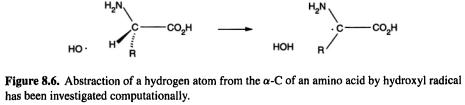
oxidation of proteins by hydroxyl radicals may initiate Alzheimer’s disease, cancer, and heart disease. The initial step in the destruction or modification of proteins by hydroxyl radical is likely to be abstraction of a hydrogen atom from the (Fig. 8.6). In a very thorough study using MP2 (section 5.4) and DFT (chapter 7), Galano et al. (2001) calculated the geometries of the species (amino acid–OH complexes, transition states, and amino acid radicals) involved in the reactions of glycine and alanine (Fig. 8.6, R–H and respectively) [20]. The rate constants were also calculated, using partition functions to calculate the preexponential factor (cf. section 5.5.2.2d). This paper provides a good account of how computational chemistry can be used to calculate absolute rate constants for reactions of molecules of moderate size.

8.1.3Concepts

There are some very basic concepts in chemistry that have proved to be helpful in rationalizing experimental facts, and which have been taught for perhaps the last fifty years, but which have nevertheless been questioned in the last decade or so; an example is the role of resonance in stabilizing species like carboxylate ions. Some newer concepts, intriguing but not as traditional, have also been scrutinized and questioned; an example is homoaromaticity.

8.1.3.1Resonance vs. inductive effects

Beginning organic chemistry students learn that carboxylic acids are stronger acids than alcohols because of resonance stabilization of the conjugate base (which is more important than the charge-separation resonance in the acid), while resonance does not figure in either an alcohol or its conjugate base. This traditional wisdom was apparently first questioned by Thomas and Siggel, on the basis of photoelectron spectroscopy [21]. They concluded that the relatively high acidity of carboxylic acids is largely inherent in the acid itself, as a consequence of the polarization of the COOH group caused by the electronegative carbonyl group pulling electrons from the hydrogen atom. This idea was taken up by Streitwieser, and applied to other acids, e.g. nitric and nitrous acids, dimethyl sulfoxide and dimethyl sulfone [22]. The results for carbonyl compounds were interpreted in accord with another iconoclastic idea, namely that the carbonyl group is better regarded as than as [23]. This polarization interpretation was arrived at largely with the aid of atoms-in-molecules (AIM) analysis of the electron populations on the atoms involved (section 5.5.4), and a simpler variation of AIM (the projection function difference plot) developed by Streitwieser and coworkers [24]. Work by others also supports the view that it is “initial-state electrostatic polarization” that is

Literature, Software, Books and Websites 453

largely responsible for the acidity of several kinds of compounds, including carboxylic acids [25]. Streitwieser cautions that “merely reproducing experiment does not teach us much unless the results are analyzed to provide understanding of the important contributions to the numbers in terms of reference systems and simpler models.” [26]. Note that such analysis is presented to a large extent visually (section 5.5.6).

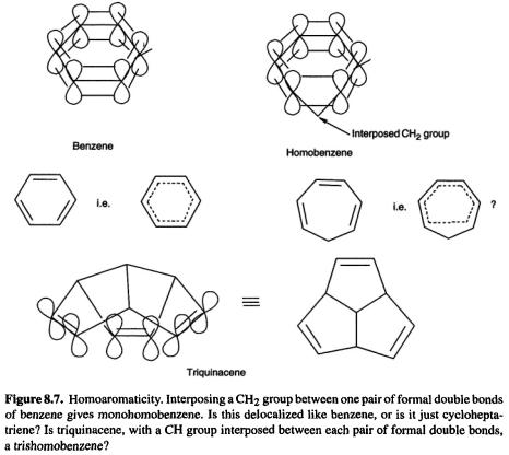
8.1.3.2Homoaromaticity

Aromaticity [27] is associated with the delocalization of (in the simplest version) electrons (the role of these electrons in imposing symmetry on the prototypical aromatic species, benzene, is being questioned, but that is another story [28]). A Hückel number of cyclically delocalized electrons confers aromaticity on a molecule (section 4.3.5). The idea behind homoaromaticity (homologous aromaticity) is that if a system is aromatic, then if we interpose one or more atoms between adjacent orbitals of the system, provided overlap is not lost, the aromaticity may persist (Fig. 8.7). While there is little doubt about the reality of homoaromaticity in ions, neutral homoaromaticity has been elusive [29].

454 Computational Chemistry

One molecule that might be expected to be homoaromatic, if the phenomenon can exist in neutral species, is triquinacene (Fig. 8.7): the three double bonds are held rigidly in an orientation which appears favorable for continuous overlap with concomitant cyclic delocalization of six electrons. Indeed, its potential aromaticity was one of the reasons cited for the synthesis of this compound [30]. A measurement of the heat of hydrogenation of triquinacene found a value lower than that for each of the next two steps (leading to hexahydrotriquinacene) [31]. This was taken as proof of homoaromaticity in the triene, i.e. 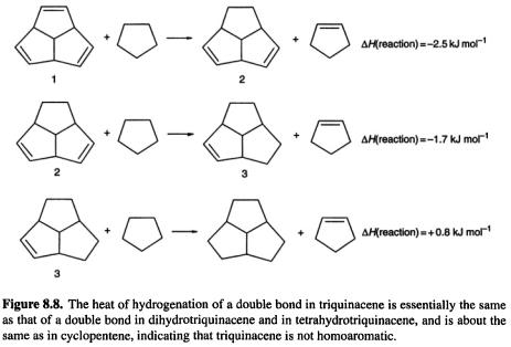that the compound was stabler than expected for an unstabilized species (note that this is a small stabilization energy compared to the resonance energy of benzene, a recent computational estimate of which is However, a recent experimental and computational study of this question led to the conclusion that triquinacene is not homoaromatic [33]. This was shown by (a) redetermination of its heat of formation (which had been calculated from the heat of hydrogenation in the earlier work [31]) using the measured heat of combustion, (b) by calculation of the heat of hydrogenation of a double bond in triquinacene and in its diand tetrahydro derivatives (1, 2, 3, Fig. 8.8), and by (c) calculation of magnetic properties of the triene and related molecules. The heat of formation was about higher than the previously reported [31] value, removing the supposed stabilization energy. The heats of hydrogenation of the double bonds were calculated with the aid of homodesmotic reactions, a kind of isodesmic reaction (section 5.5.2.2a) which preserves the number of each kind of bond, and so in which correlation errors should cancel well; for 1, 2, and 3 the calculated hydrogenation energies of a double bond are all essentially the same, showing that a double bond of 1 is an ordinary cyclopentene double bond. Note that using cyclopentane (Fig. 8.8) rather than, say, ethane – which would also preserve bond types – to (conceptually) hydrogenate 1, 2,