


Introduction to Quantum Mechanics 101
4.3.3 Matrices and determinants
Matrix algebra was invented by Cayley22 as a systematic way of dealing with systems of linear equations. The single equation in one unknown
has the solution
Consider next the system of two equations in two unknowns
22Arthur Cayley, lawyer and mathematician, born Richmond, England, 1821. Graduated Cambridge. Professor, Cambridge. After Euler and Gauss, history’s most prolific author of mathematical papers. Died Cambridge, 1895.

102 Computational Chemistry
The subscripts of the unknowns coefficients a indicate row 1, column 1, row 1, column 2, etc. We will see that using matrices the solutions (the values of x and y) can be expressed in a way analogous to that for the equation 
A matrix is a rectangular array of “elements” (numbers, derivatives, etc.) that obeys certain rules of addition, subtraction, and multiplication. Curved or angular brackets are used to denote a matrix:
or
Do not confuse matrices with determinants (below), which are written with straight lines, e.g.
is a determinant, not a matrix. This determinant represents the number 
 In contrast to a determinant, a matrix is not a number, but rather an operator (although some would consider matrices to be generalizations of numbers, with e.g. the 1 × 1 matrix
  An operator acts on a function (or a vector) to give a new function, e.g. d/dx acts on (differentiates) f (x) to give
and the square root operator acts on  to give y. When we have done matrix multiplication you will see that a matrix can act on a vector and rotate it through an angle to give a new vector.
Let us look at matrix addition, subtraction, multiplication by scalars, and matrix multiplication (multiplication of a matrix by a matrix).
Addition and subtraction
Matrices of the same size (2 × 2 and 2 × 2, 3 × 1 and 3 × 1, etc.) can be added just by adding corresponding elements:
Subtraction is similar:

Introduction to Quantum Mechanics 103
Multiplication by a scalar
A scalar is an ordinary number (in contrast to a vector or an operator), e.g. 1, 2,  1.714,
  etc. To multiply a matrix by a scalar we just multiply every element by the number:
Matrix multiplication
We could define matrix multiplication to be analogous to addition: simply multiplying corresponding elements. After all, in mathematics any rules are permitted, as long as they do not lead to contradictions. However, as we shall see in a moment, for matrices to be useful in dealing with simultaneous equations we must adopt a slightly more complex multiplication rule. The easiest way to understand matrix multiplication is to first define series multiplication. If
series |
and series |
then we define the series product as |
|
So for example, if  and
and  then
then
Now it is easy to understand matrix multiplication: if  where A, B, and C are matrices, then element i,j of the product matrix C is the series product of row i of A and column j of B. For example,
(With practice, you can multiply simple matrices in your head.) Note that matrix multiplication is not commutative: AB is not necessarily BA, e.g.
(Two matrices are identical if and only if their corresponding elements are the same.) Note that two matrices may be multiplied together only if the number of columns of the first equals the number of rows of the second. Thus we can multiply A(2 × 2)B(2 × 2), A(2 × 2)B(2 × 3), A(3 × 1)B(1 × 3), and so on. A useful mnemonic is  (a × c), meaning, for example that A(2 × 1) times B(1 × 2) gives C(2 × 2):
It is helpful to know beforehand the size, i.e. (2 × 2), (3 × 3), whatever, of the matrix you will get on multiplication.

104 Computational Chemistry
To get an idea of why matrices are useful in dealing with systems of linear equations, let us go back to our system of equations
Provided certain conditions are met this can be solved for x and y, e.g. by solving (1) for x in terms of y then substituting for x in (2) etc. Now consider the equations from the matrix viewpoint. Since
clearly AB corresponds to the left-hand side of the system, and the system can be written
A is the coefficients matrix, B is the unknowns matrix, and C is the constants matrix. Now, if we can find a matrix  such that
  (analogous to the numbers
  then
then
Thus the unknowns matrix is simply the inverse of the coefficients matrix times the
constants matrix. Note that we multiplied by |
on the left |
which |
is not the same as multiplying on the right, which would give |
this is |
|
not necessarily the same as B. |
|
|
To see that a matrix can act as an operator consider the vector from the origin to the point P(3,4). This can be written as a column matrix, and multiplying it by the rotation matrix shown transforms it (rotates it) into another matrix:
Some important kinds of matrices
These matrices are particularly important in computational chemistry:
(1)the zero matrix (the null matrix),
(2)diagonal matrices,
(3)the unit matrix (the identity matrix),
(4)the inverse of another matrix,
(5)symmetric matrices,

Introduction to Quantum Mechanics 105
(6)the transpose of another matrix,
(7)orthogonal matrices.
(1)The zero matrix or null matrix, 0, is any matrix with all its elements zero. Examples:
Clearly, multiplication by the zero matrix (when the  mnemonic permits multiplication) gives a zero matrix.
(2)A diagonal matrix is a square matrix that has all its off-diagonal elements zero; the (principal) diagonal runs from the upper left to the lower right. Examples:
(3)the unit matrix or identity matrix 1 or I is a diagonal matrix whose diagonal elements are all unity. Examples:
Since diagonal matrices are square, unit matrices must be square (but zero matrices can be any size). Clearly, multiplication (when permitted) by the unit matrix leaves the
other matrix unchanged: |
|
|
(4) The inverse |
of another matrix A is the matrix that, multiplied A, on the left |
|
or right, gives the unit matrix: |
Example: |
|
|
If |
then |
Check it out.
(5) A symmetric matrix is a square matrix for which  for each element. Examples:
Note that a symmetric matrix is unchanged by rotation about its principal diagonal. The complex-number analogue of a symmetric matrix is a Hermitian matrix (after the mathematician Charles Hermite); this has  e.g. if element
  then element
  the complex conjugate of element
  Since all the matrices we will use are real rather than complex, attention has been focussed on real matrices here.

106Computational Chemistry
(6)The transpose  or
or  of a matrix A is made by exchanging rows and columns. Examples:
If |
then |
If |
then |
Note that the transpose arises from twisting the matrix around to interchange rows and columns. Clearly the transpose of a symmetric matrix A is the same matrix A. For complex-number matrices, the analogue of the transpose is the conjugate transpose  to get this form
  the complex conjugate of A, by converting each complex number element a + bi in A to its complex conjugate a – bi, then switch the rows and columns of
  to get
  Physicists call
  the adjoint of A, but mathematicians use adjoint to mean something else.
(7) An orthogonal matrix is a square matrix whose inverse is its transpose: if 
 then A is orthogonal. Examples:
We saw that for the inverse of a matrix, . so for an orthogonal matrix
  since here the transpose is the inverse. Check this out for the matrices shown. The complex analogue of an orthogonal matrix is a unitary matrix; its inverse is its conjugate transpose.
The columns of an orthonormal matrix are orthonormal vectors. This means that if we let each column represent a vector, then these vectors are mutually orthogonal and each one is normalized. Two or more vectors are orthogonal if they are mutually perpendicular (i.e. at right angles), and a vector is normalized if it is of unit length. Consider the matrix  above. If column 1 represents the vector
  and column 2 the vector
  then we can picture these vectors like this (the long side of a right triangle is of unit length if the squares of the other sides sum to 1):
The two vectors are orthogonal: from the diagram the angle between them is clearly 90° since the angle each makes with, say, the x-axis is 45°. Alternatively, the angle can

Introduction to Quantum Mechanics 107
be calculated from vector algebra: the dot product (scalar product) is
where  (“mod v”) is the absolute value of the vector, i.e. its length:
(or  for a 3D vector).
Each vector is normalized, i.e.
The dot product is also
(with an obvious extension to 3D space)
i.e.
and so
Likewise, the three columns of the matrix  above represent three mutually perpendicular, normalized vectors in 3D space. A better name for an orthogonal matrix would be an orthonormal matrix. Orthogonal matrices are important in computational chemistry because MOs can be regarded as orthonormal vectors in a generalized n-dimensional space (Hilbert space, after the mathematician David Hilbert). We extract information about MOs from matrices with the aid of matrix diagonalization.
Matrix diagonalization
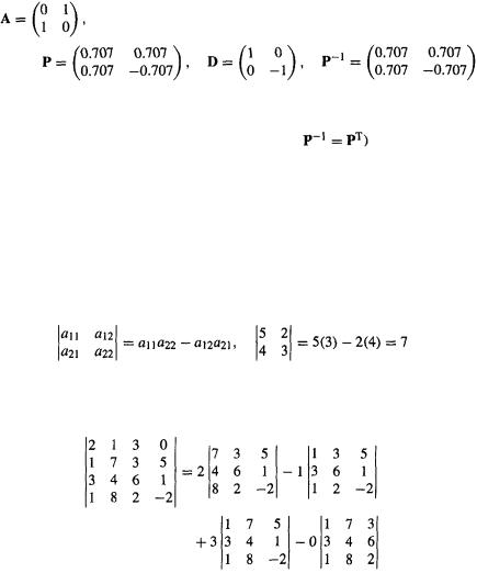
Modern computer programs use matrix diagonalization to calculate the energies (eigenvalues) of MOs and the sets of coefficients (eigenvectors) that help define their size and shape. We met these terms, and matrix diagonalization, briefly in section 2.5; “eigen” means suitable or appropriate, and we want solutions of the Schrödinger equation that are appropriate to our particular problem. If a matrix A can be written 
where D is a diagonal matrix (you could call P and  preand postmultiplying matrices), then we say that A is diagonalizable (can be diagonalized). The process of finding P and D (getting
  from P is simple for the matrices of computational chemistry – see below) is matrix diagonalization. For example,
if
then |
and |
Check it out. Linear algebra texts describe an analytical procedure using determinants, but computational chemistry employs a numerical iterative procedure called Jacobi matrix diagonalization, or some related method, in which the off-diagonal elements are made to approach zero.
108 Computational Chemistry
Now, it can be proved that if and only if A is a symmetric matrix (or more generally, if we are using complex numbers, a Hermitian matrix – see symmetric matrices, above), then P is orthogonal (or more generally, unitary – see orthogonal matrices, above) and so the inverse  of the premultiplying matrix P is simply the transpose of
  (or more generally, what computational chemists call the conjugate transpose
  see transpose, above). Thus
if
then
(In this simple example the transpose of P happens to be identical with P.) In the spirit of numerical methods 0.707 is used instead of  A matrix like A above, for which the
premultiplying matrix P is orthogonal (and so for which is said to be orthogonally diagonalizable. The matrices we will use to get MO eigenvalues and eigenvectors are orthogonally diagonalizable. A matrix is orthogonally diagonalizable if and only if it is symmetric; this has been described as “one of the most amazing theorems in linear algebra” (see S. Roman, “An Introduction to Linear Algebra with Applications", Harcourt Brace, 1988, p. 408) because the concept of orthogonal diagonalizability is not simple, but that of a symmetric matrix is very simple.
Determinants
A determinant is a square array of elements that is a shorthand way of writing a sum of products; if the elements are numbers, then the determinant is a number. Examples:
As shown here, a 2 × 2 determinant can be expanded to show the sum it represents by “cross multiplication.” A higher-order determinant can be expanded by reducing it to smaller determinants until we reach 2 × 2 determinants; this is done like this:
Here we started with element (1, 1) and moved across the first row. The first of the above four terms is 2 times the determinant formed by striking out the row and column in which 2 lies, the second term is minus 1 times the determinant formed by striking out the row and column in which 1 lies, the third term is plus 3 times the determinant formed by striking out the row and column in which 3 lies, and the fourth term is minus 0 times the determinant formed by striking out the row and column in which 0 lies; thus starting with the element of row 1, column 1, we move along the row and multiply by +1,