

Chapter 4
Introduction to Quantum Mechanics in Computational Chemistry
It is by logic that we prove, but by intuition that we discover.
J. H. Poincaré, ca. 1900.
4.1 PERSPECTIVE
Chapter 1 outlined the tools that computational chemists have at their disposal, chapter 2 set the stage for the application of these tools to the exploration of potential energy surfaces, and chapter 3 introduced one of these tools, molecular mechanics. In this chapter you will be introduced to quantum mechanics, and to quantum chemistry, the application of quantum mechanics to chemistry. Molecular mechanics is based on classical physics, physics before modern physics; one of the cornerstones of modern physics is quantum mechanics, and ab initio (chapter 5), semiempirical (SE) (chapter 6), and density functional (chapter 7) methods belong to quantum chemistry. This chapter is designed to ease the way to an understanding of the role of quantum mechanics in computational chemistry. The word quantum comes from Latin (quantus, “how much?”, plural quanta) and was first used in our sense by Max Planck in 1900, as an adjective and noun, to denote the constrained quantities or amounts in which energy can be emitted or absorbed. Although the term quantum mechanics was apparently first used by Born (of the Born–Oppenheimer approximation, section 2.3) in 1924, in contrast to classical mechanics, the matrix algebra and differential equation techniques that we now associate with the term were presented in 1925 and 1926 (section 4.2.6).
“Mechanics” as used in physics is traditionally the study of the behavior of bodies under the action of forces like, e.g. gravity (celestial mechanics). Molecules are made of nuclei and electrons, and quantum chemistry deals, fundamentally, with the motion of electrons under the influence of the electromagnetic force exerted by nuclear charges. An understanding of the behavior of electrons in molecules, and thus of the structures and reactions of molecules, rests on quantum mechanics and in particular on that adornment of quantum chemistry, the Schrödinger equation. For that reason we will consider in outline the development of quantum mechanics leading up to the

82 Computational Chemistry
Schrödinger equation, and then the birth of quantum chemistry with (at least as far as molecules of reasonable size goes) the application of the Schrödinger equation to chemistry by Hückel. This simple Hückel method is currently disdained by some theoreticians, but its discussion here is justified by the fact that (1) it continues to be useful in research and (2) it “is immensely useful as a model, today . . . because it is the model which preserves the ultimate physics, that of nodes in wave functions. It is the model which throws away absolutely everything except the last bit, the only thing that if thrown away would leave nothing. So it provides fundamental understanding.”1 A discussion of a generalization of the simple Hückel method, the extended Hückel method, sets the stage for chapter 5. The historical approach used here, although perforce somewhat superficial, may help to ameliorate the apparent arbitrariness of certain features of quantum chemistry [1,2]. An excellent introduction to quantum chemistry is the text by Levine [3].
Our survey of the factors that led to modern physics and quantum chemistry will follow the sequence:
(1)the origins of quantum theory: blackbody radiation and the photoelectric effect;
(2)radioactivity (brief);
(3)relativity (very brief);
(4)the nuclear atom;
(5)the Bohr atom;
(6)the wave mechanical atom and the Schrödinger equation.
4.2THE DEVELOPMENT OF QUANTUM MECHANICS (THE SCHRÖDINGER EQUATION)
4.2.1The origins of quantum theory: blackbody radiation and the photoelectric effect
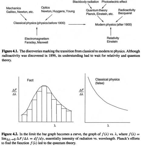
Three discoveries mark the transition from classical to modern physics: quantum theory, radioactivity, and relativity (Fig. 4.1). Quantum theory had its origin in the study of blackbody radiation and the photoelectric effect.
Blackbody radiation
A blackbody is one that is a perfect absorber of radiation: it absorbs all the radiation falling on it, without reflecting any. More relevant for us, the radiation emitted by a hot blackbody depends (as far as the distribution of energy with wavelength goes) only on the temperature, not on the material the body is made of, and is thus amenable to relatively simple analysis. The sun is approximately a blackbody; in the lab a good source of blackbody radiation is a furnace with blackened insides and a small aperture for the radiation to escape. In the second half of the nineteenth century the distribution of
1 Personal communication from Professor Roald Hoffmann (see the extended Hückel method, section 4.4).
Introduction to Quantum Mechanics 83
energy with respect to wavelength that characterizes blackbody radiation was studied, in research that is associated mainly with Lummer and Pringsheim [1]. They plotted the flux  (in modern SI units,
 per wavelength emitted by a blackbody over a wavelength range
  vs. the wavelength, for various temperatures (Fig. 4.2):
  The result is a histogram or bar graph in which the area of each rectangle is
  and represents the flux (energy per second per unit area) emitted in the wavelength range covered by that
  can be called the flux density for that particular wavelength range
  The total area of all the rectangles is the total flux emitted over its whole wavelength range by the blackbody. As
  approaches zero (note that for the nonmonochromatic radiation from a blackbody the flux at a particular wavelength is essentially zero) the histogram approaches being a smooth curve, the ratio of finite increments approximates a derivative, and we can ask: what is the function (Fig. 4.2)
 In the answer to this question lay the beginnings of quantum theory.

84 Computational Chemistry
Late nineteenth century physics, classical physics at its zenith, predicted that the flux density emitted by a black body should rise without limit as the wavelength decreases. This is because classical physics held that radiation of a particular frequency was emitted by oscillators (atoms or whatever) vibrating with that frequency, and that the average energy of an oscillator was independent of its frequency; since the number of possible frequencies increases without limit, the flux density (energy per second per unit area per wavelength interval) from the blackbody should rise without limit toward higher frequencies or shorter wavelengths, into the ultraviolet, and so the total flux (energy per second per unit area) should be infinite. This is clearly absurd and was recognized as being absurd; in fact, it was called “the ultraviolet catastrophe” [1]. To understand the nature of blackbody radiation and to escape the ultraviolet catastrophe, physicists in the 1890s tried to find the function (Fig. 4.2) 
Without breaking with classical physics, Wien had found a theoretical equation that fit the Lummer–Pringsheim curve at relatively short wavelengths, and Rayleigh and Jeans
one that fit at relatively long wavelengths. |
adopted a different approach: |
he found, in 1900, a purely empirical equation |
that fit the facts, and then |
tried to interpret the equation theoretically. To do this he had to make two assumptions:
(1)the total energy possessed by the oscillators in the frequency range  is the Greek letter nu, commonly used for frequency, not to be confused with
  vee, commonly used for velocity) is proportional to the frequency:
(2)the emission or absorption of radiation of frequency  by the collection of oscillators is caused by jumps between energy levels, with loss or gain of a quantity of energy
The constant k, now recognized as a fundamental constant of nature, 6.626 × 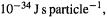 is called Planck’s constant, and is denoted by h, so Eq. (4.2) becomes
Why the letter h? Evidently because h is sometimes used in mathematics to denote infinitesimals and Planck intended to let this quantity go to zero. In the event, it turned out to be small but finite. Apparently the letter was first used to denote the new constant in a talk given by Planck at a meeting (Sitzung) of the German Physical Society in Berlin, on 14 December 1900 [4]. The interpretation of Eq. (4.3), a fundamental equation of quantum theory, as meaning that the energy represented by radiation of frequency v is absorbed and emitted in quantized amounts hv (definite, constrained amounts; jerkily rather than continuously) was, ironically, apparently never fully accepted by Planck [5]. Planck’s constant is a measure of the graininess of our universe: because it is so small processes involving energy changes often seem to take place smoothly,
2 Max Planck, born Kiel, Germany, 1858. Ph.D. Berlin 1879. Professor, Kiel, Berlin. Nobel prize in physics for quantum theory of blackbody radiation 1918. Died Göttingen, 1947.

Introduction to Quantum Mechanics 85
but on an ultramicroscopic scale the graininess is there [6]. The constant h is the hallmark of quantum expressions, and its finite value distinguishes our universe from a nonquantum one.
The photoelectric effect
An apparently quite separate (but in science no two phenomena are really ever unrelated) phenomenon that led to Eq. (4.3), which is to say to quantum theory, is the photoelectric effect: the ejection of electrons from a metal surface exposed to light. The first inkling of this phenomenon was due to Hertz,3 who in 1888 noticed that the potential needed to elicit a spark across two electrodes decreased when ultraviolet light shone on the negative electrode. Beginning in 1902, the photoelectric effect was first studied systematically by Lenard,4 who showed that the phenomenon observed by Hertz was due to electron emission.
Facts (Fig. 4.3) that classical physics could not explain were the existence of a threshold frequency for electron ejection, that the kinetic energy of the electrons is linearly related to the frequency of the light, and the fact that the electron flux (electrons per unit area per second) is proportional to the intensity of the light. Classical physics predicted that the electron flux should be proportional to the light frequency, decreasing with a decrease in frequency, but without sharply falling to zero below a certain frequency, and that the kinetic energy of the electrons should be proportional to the intensity of the light, not the frequency.
These facts were explained by Einstein5 in 1905 in a way that now appears very simple, but in fact relies on concepts that were at the time revolutionary. Einstein went beyond Planck and postulated that not only was the process of absorption and emission of light quantized, but that light itself was quantized, consisting of in effect of particles of energy
where  is the frequency of the light. These particles were given the name photons (Arthur Compton, ca. 1923). If the energy of the photon before it removes an electron from the metal is equal to the energy required to tear the electron free of the metal, plus the kinetic energy of the free electron, then
where W is the work function of the metal, energy needed to remove an electron (with no energy left over),  is the mass of an electron,
  is the velocity of electron ejected by
3Heinrich Hertz, born Hamburg, Germany, 1857. Ph.D. Berlin, 1880. Professor, Karlsruhe, Bonn. Discoverer of radio waves. Died Bonn, 1894.
4 Philipp Lenard, German physicist, born Pozsony, Austria–Hungary (now Bratislava, Slovakia), 1862. Ph.D. Heidelberg 1886. Professor, Heidelberg. Nobel prize in physics 1905, for work on cathode rays. Lenard supported the Nazis and rejected Einstein’s theory of relativity. Died Messelhausen, Germany, 1947.
5Albert Einstein, German–Swiss–American physicist. Born Ulm, Germany, 1879. Ph.D. Zürich 1905. Professor Zürich, Prague, Berlin; Institute for Advanced Studies, Princeton, New Jersey. Nobel Prize in physics 1921 for theory of the photoelectric effect. Best known for the special (1905) and general (1915) theories of relativity. Died Princeton, 1955.