

176 Computational Chemistry
5.2.3.5The meaning of the HF equations
The HF equations (5.47) (in matrix form Eqs (5.44) and (5.46)) are pseudoeigenvalue equations asserting that the Fock operator  acts on a wavefunction
  to generate an energy value
  times
times  Pseudoeigenvalue because, as stated above, in a true eigenvalue equation the operator is not dependent on the function on which it acts; in the HF equations
  depends on
  because (Eq. (5.36)) the operator contains
  and
and  which in turn depend (Eqs (5.29) and (5.30)) on
  Each of the equations in the set (5.47) is for a single electron (“electron one” is indicated, but any ordinal number could be used), so the HF operator
  is a one-electron operator, and each spatial molecular orbital
  is a one-electron function (of the coordinates of the electron). Two electrons can be placed in a spatial orbital because the full description of each of these electrons requires a spin /unction
  or
or (section 5.2.3.1) and each electron “moves in” a different spin orbital. The result is that the two electrons in the spatial orbital
  do not have all four quantum numbers the same (for an atomic
  orbital, e.g. one electron has quantum numbers n = 1, l= 0, m= 0 and
  while the other has n= 1, l = 0, m = 0 and
and so the Pauli exclusion principle is not violated.
The functions  are the spatial molecular (or atomic) orbitals or wavefunctions that (along with the spin functions) make up the overall or total molecular (or atomic) wavefunction
 which can be written as a Slater determinant (Eq. (5.12)). Concerning the energies
  from the fact that
(this follows simply from multiplying both sides of a HF equation by  and integrating, noting that
  is normalized) and the definition of
  (Eq. (5.36)) we get
i.e.
(the operators  and
and  in Eq. (5.36) have been transformed by integration into the integrals J and K in Eq. 5.49)). Equation (5.50) shows that
 is the energy of an electron in
  subject to interaction with all the other electrons in the molecule:
  Eq. (5.19) is the energy of the electron due only to its motion (kinetic energy) and to the attraction of the nuclear core (electron-nucleus potential energy), while the sum of 2J–K terms represents the exchange-corrected (via K) coulombic repulsion (through J) energy resulting from the interaction of the electron with all the other electrons in the molecule or atom [17].
In principle the Eqs (5.47) allow us to calculate the molecular orbitals (MOs)  and the energy levels
  We could start with “guesses” (actually obtained by intuition or analogy) of the MOs (the zeroth approximation to these) and use these to construct the
|
Ab initio calculations 177 |
operator |
(Eq. (5.36), then allow to operate on the guesses to yield energy levels |
(the first approximation to the ) and new, improved [18] functions (the first calculated |
|||
approximations to the |
Using the improved functions in and operating on these |
||
gives the second approximations to the |
and |
and the process is continued until |
|
 and
and  no longer change (within preset limits), which occurs when the smeared-out electrostatic field represented in Eq. (5.17) by
  (cf. Fig. 5.3) ceases to change appreciably – is consistent from one iteration cycle to the next, i.e. is selfconsistent. This is, of course, in exactly the same spirit as the procedure described in section 5.2.2 using the Hartree product as our total or overall wavefunction
  The main difference between the two methods is that the HF method represents
 as a Slater determinant of component spin MOs rather than as a simple product of spatial MOs, and a consequence of this is that the calculation of the average coulombic field in the Hartree method involves only the coulomb integral J, but in the HF modification we need the coulomb integral J and the exchange integral K, which arises from Slater determinant terms that differ in exchange of electrons. Because K acts as a kind of “Pauli correction” to the classical electrostatic repulsion, reminding the electrons that two of them of the same spin cannot occupy the same spatial orbital, electron–electron repulsion is less in the HF method than if a simple Hartree product were used. Of course K does not
arise in calculations involving no electrons of like spin, as in |
or (section 4.4.1; also |
||||
section 5.4.3.6e) |
which have only two, paired-spin, electrons. At the end of |
||||
the iterative procedure we have the MO’s |
and their corresponding energy levels |
||||
and the total wavefunction |
the Slater determinant of the |
The |
can be used |
||
to calculate the total electronic energy of the molecule, and the MO’s |
areuseful |
||||
heuristic approximations to the electron distribution, while the total wavefunction  can in principle be used to calculate anything about the molecule. Applications of the energy levels and the MO’s are given in section 5.4.
5.2.3.6Basis functions and the Roothaan–Hall equations
5.2.3.6a Deriving the Roothaan–Hall equations
As they stand, the HF equations (5.44), (5.46) or (5.47) are not very useful for molecular calculations, mainly because (1) they do not prescribe a mathematically viable procedure getting the initial guesses for the MO wavefunctions  which we need to initiate the iterative process (section 5.2.3.5), and (2) the wavefunctions may be so complicated that they contribute nothing to a qualitative understanding of the electron distribution. For calculations on atoms, which obviously have much simpler orbitals than molecules, we could use for the
  atomic orbital wavefunctions based on the solution of the Schrödinger equation for the hydrogen atom (taking into account the increase of atomic number and the screening effect of inner electrons on outer ones [19]). This yields the atomic wavefunctions as tables of
  at various distances from the nucleus. This is not a suitable approach for molecules because among molecules there is no prototype species occupying a place analogous to that of the hydrogen atom in the hierarchy of atoms, and as indicated above it does not readily lend itself to an interpretation of how molecular properties arise from the nature of the constituent atoms.
178 Computational Chemistry
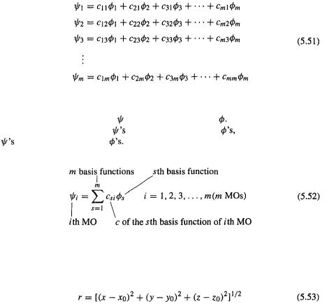
In 1951 Roothaan and Hall independently pointed out [20] that these problems can be solved by representing MOs as linear combinations of basis functions (just as in the SHM, in chapter 4, the  MOs are constructed from atomic p orbitals). For a basis-function expansion of MOs we write
In devising a more compact notation for this set of equations it is very helpful, particularly when we come to the matrix treatment in section 5.2.3.6c, to use different
subscripts to denote the MOs |
and the basis functions |
Conventionally, |
Roman |
letters have been used for the |
and Greek letters for the |
or i, j, k, l, … for the |
|
and r, s, t, u,... for the |
The latter convention will be adopted here, |
and we |
|
can write the Eqs (5.51) as |
|
|
|
We are expanding each MO  in terms of m basis functions. The basis functions are usually (but not necessarily) located on atoms, i.e. for the function
  (x, y, z), where x, y, z are the coordinates of the electron being treated by this one-electron function, the distance of the electron from the nucleus is:
where  are the coordinates of the atomic nucleus in the coordinate system used to define the geometry of the molecule. Because each basis function may usually be regarded (at least vaguely) as some kind of atomic orbital, this linear combination of basis functions approach is commonly called a linear combination of atomic orbitals (LCAO) representation of the MOs, as in the SHM and EHM (sections 4.3.3 and 4.4.1). The set of basis functions used for a particular calculation is called the basis set.
We need at least enough spatial MOs  to accommodate all the electrons in the molecule, i.e. we need at least n
  for the 2n electrons (recall that we are dealing with closed-shell molecules). This is ensured because even the smallest basis sets used in ab initio calculations have for each atom at least one basis function corresponding to each orbital conventionally used to describe the chemistry of the atom, and the number of basis functions
  is equal to the number of (spatial) MOs
  (section 4.3.4). An example will make this clear: for an ab initio calculation on
  the smallest basis
Ab initio calculations 179
set would specify for  and for each
  These nine basis functions
  (5 on C and 4 × 1 = 4 on H) create nine spatial MO’s
  which could hold 18 electrons; for the 10 electrons of
  we need only 5 spatial MO’s. There is no upper limit to the size of a basis set: there are commonly many more basis functions, and hence MOs, than are needed to hold all the electrons, so that there are usually many unoccupied MO’s. In other words, the number of basis functions m in the expansions (5.52) can be much bigger than the number n of pairs of electrons in the molecule, although only the n occupied spatial orbitals are used to construct the Slater determinant which represents the HF wavefunction (section 5.2.3.1). This point, and basis sets, are discussed further in section 5.3.
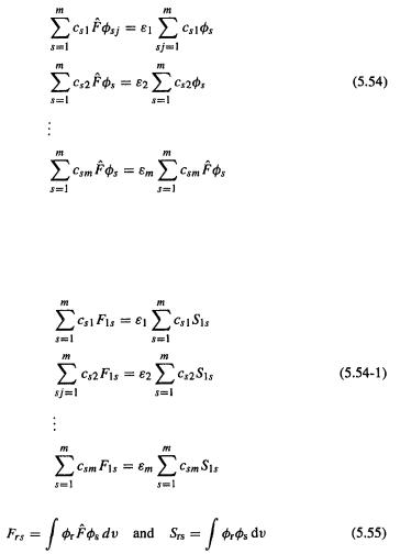
To continue with the Roothaan–Hall approach, we substitute the expansion (5.52) for the  into the HF equations (5.47), getting (we will work with m, not n, HF equations since there is one such equation for each MO, and our m basis functions will generate m MOs):
( operates on the functions
  not on the c’s, which have no variables x, y, z). Multiplying each of these m equations by
  (or
(or  etc. if the
  are complex functions, as is occasionally the case) and integrating, we get m sets of equations (one for each of the basis functions
  Basis function
  gives
gives
where
180 Computational Chemistry
Basis function  gives
gives
Finally, basis function  gives
gives
In the m sets of equations (5.54-1) to (5.54-m) each set itself contains m equations (the subscript of  for example, runs from 1 to m), for a total of m × m equations. These equations are the Roothaan-Hall version of the HF equations; they were obtained by substituting for the MOs
  in the HF equations a linear combination of basis functions
  weighted by c’s). The Roothaan–Hall equations are usually written more compactly, as
We have m × m equations because each of the m spatial MO’s |
we used (recall that |
|||||
there is one HF equation for each |
Eqs (5.47)) is expanded with m basis functions. |
|||||
The Roothaan–Hall equations connect the basis functions |
(contained in the integrals |
|||||
F and S, Eqs (5.55)), the coefficients c, and the MO energy levels |
Given a basis |
|||||
set |
s = 1, 2, 3, …, m} they can be used to calculate the c’s, and thus the MOs |
|||||
(Eq. (5.52)) and the MO energy levels |
The overall electron distribution in the |
|||||
molecule can be calculated from the total wavefunction |
which can be written as |
|||||
a Slater determinant of the “component” spatial wavefunctions |
(by including spin |
|||||
functions), and in principle anyway, |
any property of a molecule can be calculated |
|||||
Ab initio calculations 181
from The componentwavefunctions
  and their energy levels
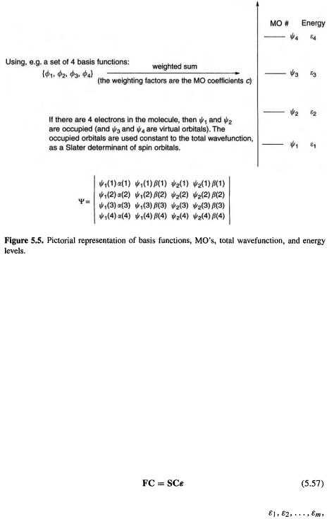
 are extremely useful, as chemists rely heavily on concepts like the shape and energies of, for example, the HOMO and LUMO of a molecule (MO concepts are reviewed in chapter 4). The energy levels enable (with a correction term) the total energy of a molecule to be calculated, and so the energies of molecules can be compared and reaction energies and activation energies can be calculated. The Roothaan–Hall equations, then, are a cornerstone of modern ab initio calculations, and the procedure for solving them is outlined next. These ideas are summarized pictorially in Fig. 5.5.
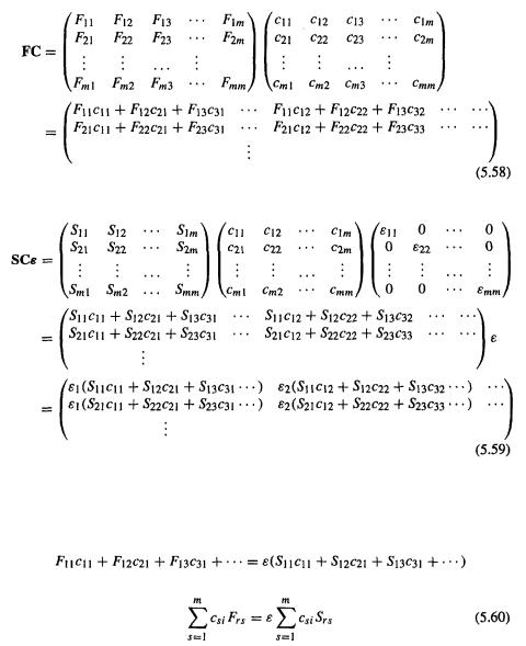
The fact that the Roothaan–Hall equations (5.56) are actually a total of m × m equations suggests that they might be expressible as a single matrix equation, since the single matrix equation AB = 0, where A and B are m × m matrices, represents m × m “simple” equations, one for each element of the product matrix AB (work it out for two 2 × 2 matrices). A single matrix equation would be easier to work with than  equations and might allow us to invoke matrix diagonalization as in the case of the simple and extended Hückel methods (sections 4.3.3 and 4.4.1). To subsume the sets of Eqs (5.54-1) to (5.54-m), i.e. Eqs (5.56), into one matrix equation, we might (eschewing a rigorous deductive approach) suspect that the matrix form is the rather obvious possibility
Here F, C and S would have to be m × m matrices, since there are  and S’s, and
  would be an m × m diagonal matrix with the nonzero elements
182 Computational Chemistry
since  must contain only m elements, but has to be m × m to make the right-hand side matrix product the same size as that on the left.
This is easily checked: the left-hand side of Eq. (5.57) is
The right-hand side of Eq. (5.57) is
Now compare FC (5.58) and  (5.59). Comparing element
  of FC (multiplied out to give a single matrix as shown in (5.58)) with element
  of
of (multiplied out to give a single matrix as shown in (5.59)) we see that if
  i.e. if (5.57) is true, then
i.e.
But this is the first equation of the set (5.53-1). Continuing in this way we see that matching each element of (the multiplied-out) matrix FC (5.58) with the corresponding element of (the multiplied-out) matrix  gives one of the equations of the set (5.54-1) to (5.54-m), i.e. of the set (5.56). This can be so only if
  so this matrix equation is indeed equivalent to the set of Eqs (5.56).
Ab initio calculations 183
Now we have  the matrix form of the Roothaan–Hall equations. These equations are sometimes called the Hartree–Fock–Roothaan equations, and, often, the Roothaan equations, as Roothaan’s exposition was the more detailed and addresses itself more clearly to a general treatment of molecules. Before showing how they are used to do ab initio calculations, a brief review of how we got these equations is in order.
Summary of the derivation of the Roothaan–Hall equations:
1.The total wavefunction of an atom or molecule was expressed as a Slater determinant of spin MOs
  (spatial)
  and
and  (spatial)
  Eq. (5.12).
2.From the Schrödinger equation we got an expression for the electronic energy of the atom or molecule,  Eq. (5.14).
3.Substituting the Slater determinant for  and the explicit form of the Hamiltonian operator
  into (5.14) gave the energy in terms of the spatial MO’s
  (Eq. (5.17):
4. Minimizing E in (5.17) with respect to the |
(to find the best |
gave the HF |
||
equations |
(5.44). |
|
|
|
5. Substituting into the HFequations |
(5.44) the Roothaan–Hall linear com- |
|||
bination of basis functions (LCAO) |
expansions |
(5.52) for the MO’s |
||
gave the Roothaan–Hall equations (Eqs (5.56)), which can be written compactly |
||||
as |
(Eqs (5.57)). |
|
|
|
5.2.3.6b Using the Roothaan–Hall equations to do ab initio calculations – theSCFprocedure
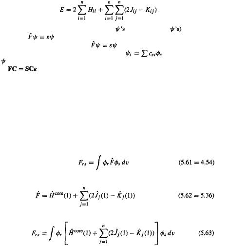
The Roothaan–Hall equations  (Eqs (5.57)) (F, C, S and
  are defined in connection with Eqs (5.58) and (5.59); the matrix elements F and S are defined by Eqs (5.54) and (5.55)) are of the same matrix form as Eq. (4.54),
  in the simple Hückel method (section 4.3.3) and the extended Hückel (section 4.4.1) method. Here, however, we have seen (in outline) how the equation may be rigorously derived. Also, unlike the case in the Hückel methods the Fock matrix elements are rigorously defined theoretically: from Eqs (5.55)
and Eq. (5.36)
it follows that
184 Computational Chemistry
where
and
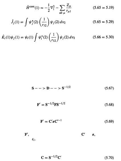
To use The Roothaan–Hall equations we want them in standard eigenvalue-like form so that we can diagonalize the Fock matrix F of Eq. (5.57) to get the coefficients c and the energy levels just as we did in connection with the extended Hückel method (section 4.4.1). The procedure for diagonalizing F and extracting the c’s and
  and is exactly the same as that explained for the extended Hückel method (although here the cycle is iterative, i.e. repetitive, see below):
1. The overlap matrix S is calculated and used to calculate an orthogonalizing matrix  as in Eqs (4.107) and (4.108):
2. is used to convert F to
  (cf. (4.104):
The transformed Fock matrix  satisfies
(cf. Eq. (4.106)). The overlap matrix S is readily calculated, so if Fcan be calculated
it can be transformed to |
which can be diagonalized to give |
and which latter |
yields the MO energy levels |
|
|
3.Transformation of  to C (Eq. (4.102)) gives the coefficients
  in the expansion of the MO’s
  in terms of basis functions
Equations (5.63)–(5.66) show that to calculate F, i.e. each of the matrix elements F, we need the wavefunctions  because
  and
and  the coulomb and exchange operators (Eqs (5.65) and (5.66)), are defined in terms of the
  It looks like we are faced with a dilemma: the point of calculating F is to get (besides the
  the
the  (the c’s with the chosen basis set
  make up the
  but to get F we need the
  The way out of this is to start with a set of approximate c’s, e.g. from an extended Hückel calculation, which needs no c’s to begin with because the extended Hückel “Fock” matrix elements are calculated from experimental ionization potentials (section 4.4.1). These c’s, the initial guess, are used with the basis functions
  to in effect (section 5.2.3.6c) calculate initial MO wavefunctions
 which are used to calculate the F elements
  Transformation
|
|
|
|
|
Ab initio calculations |
185 |
of F to |
and diagonalization gives a “first-cycle” set of |
and (after transformation |
||||
of |
to |
C) a first-cycle set of c’s. These c’s are used |
to calculate new |
i.e. a |
||
new F, and this gives a second-cycle set of |
and c’s. The process is continued until |
|||||
things – the |
the c’s (as the density matrix – section 5.2.3.6c), the energy, or, more |
|||||
usually, some combination of these – stop changing within certain pre-defined limits, i.e. until the cycles have essentially converged on the limiting  and c’s. Typically, about ten cycles are needed to achieve convergence. It is because the operator
  depends on the functions
  on which it acts, making an iterative approach necessary, that the Roothaan–Hall equations, like the HF equations, are called pseudoeigenvalue (see end of section 5.2.3.4 and start of 5.2.3.5).
Now, in the HF method (the Roothaan–Hall equations represent one implementation of the HF method) each electron moves in an average field due to all the other electrons (see the discussion in connection with Fig. 5.3, section 5.2.3.2). As the c’s are refined the MO wavefunctions improve and so this average field that each electron feels improves (since J and K, although not explicitly calculated (section 5.2.3.6c) improve with the  When the c’s no longer change the field represented by this last set of c’s is (practically) the same as that of the previous cycle, i.e. the two fields are “consistent” with one another, i.e. “self-consistent”. This Roothaan–Hall–Hartree–Fock iterative process (initial guess, first F, first-cycle c’s, second F, second-cycle c’s, third F, etc.) is therefore a self-consistent-field-procedure or SCF procedure, like the HF procedure of section 5.2.2. The terms “HF calculations/method” and “SCF calculations/method" are in practice synonymous. The key point to the iterative nature ofthe SCF procedure is that to get the c’s (for the MOs
  and the MO
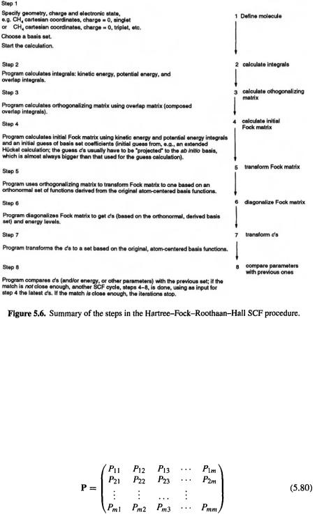
 we diagonalize a Fock matrix F, but to calculate F we need an initial guess for the c’s and we then improve the c’s by repeatedly recalculating and diagonalizing F. The procedure is summarized in Fig. 5.6. Note that in the simple and extended Hückel methods we do not need the c’s to calculate F, and there is no iterative refinement of the c’s, so these are not SCF methods; other semiempirical procedures, however (chapter 6) do use the SCF approach.
5.2.3.6c Using the Roothaan–Hall equations to do ab initio calculations – the equations in terms of the c’s and  of the LCAO expansion
The key process in the HF ab initio calculation of energies and wavefunctions is
calculation of the Fock matrix, |
i.e. of the matrix elements |
(section 5.2,3.6b). |
||
Equation (5.63) expresses these in terms of the basis functions |
and the operators |
|||
and |
but the and |
operators (Eqs (5.28) and (5.31)) are themselves func- |
||
tions of the MO’s and therefore of the c’s and the basis functions |
Obviously the |
|||
can be written explicitly in terms of the c’s and |
such a formulation enables the Fock |
|||
matrix to be efficiently calculated from the coefficients and the basis functions without explicitly evaluating the operators  and
and  after each iteration. This more explicit (in terms of the Roothaan–Hall LCAO approach) formulation of the Fock matrix will now be explained.
To see more clearly what is required, write Eq. (5.63) as
186 Computational Chemistry
using the compact Dirac notation. The operator  involves only the Laplacian differentiation operator, atomic numbers and electron coordinates, so we do not have to consider substituting the Roothaan–Hall c’s and
  into
into  The operators
 and
and  , however, invoke the integrals
  and We now examine these two integrals.
Substituting for  the basis function expansion
  and for
  (2) the expansion
 (cf. Eq. (5.52)):
where the double sum arises because we multiply the sum by the
  sum. To get the desired expression for
 we multiply this by
  and integrate with respect to the coordinates of electron 1, getting:
Note that this is really a sixfold integral, since there are three variables  for electron 1, and three
  for electron 2, represented by
  and
and  respectively. This equation can be written more compactly as
The notation
is a common shorthand for this kind of integral, which is called a two-electron repulsion integral (or two-electron integral, or electron repulsion integral); the physical significance of these is outlined in section 5.2.3.6d). This parentheses notation should not be confused with the Dirac bra-ket notation,  (a bra) and
  a ket: by definition
so
Actually, several notations have been used for the integrals of Eq. (5.73) and for other integrals; make sure to ascertain which symbolism a particular author is using.
Ab initio calculations 187
 from Eq. (5.66):
Substituting for  the basis function expansion
  and for
  the expansion
  (cf. Eq. (5.52)):
To get the desired expression for  we multiply this by
  and integrate with respect to the coordinates of electron 1:
which can be written more compactly as
where of course (cf. (5.73)) |
|
|
||
Substituting Eqs (5.72) and (5.76) for |
and |
into |
||
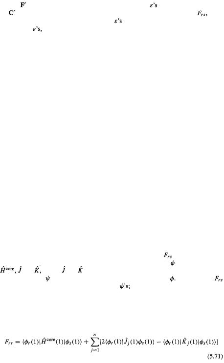
Eq. (5.71) for |
we get |
|
|
|
i.e. |
|
|
|
|
where the integral of the operator |
over the basis functions has been written as: |
|||
with |
defined by Eq. (5.64). |
|
|
|
Equation (5.78), with its ancillary definitions Eqs (5.73), (5.77), and (5.79), is what we wanted: the Fock matrix elements in terms of the basis functions  and their weighting coefficients c, for a closed-shell molecule; m is the number ofbasis functions and 2n is the number of electrons. We can use Eq. (5.78) to calculate MO’s and energy levels
188 Computational Chemistry
(section 5.2.3.6b). Given a basis set and molecular geometry (the integrals depend on molecular geometry, as will be illustrated) and starting with an initial guess at the c’s, one (or rather the computer algorithm) calculates the matrix elements  assembles them into the Fock matrix F, etc. (section 5.2.3.6b and Fig. 5.6) Let us now examine certain details connected with Eq. (5.78) and this procedure.
5.2.3.6d Using the Roothaan–Hall equations to do ab initio calculations – some details
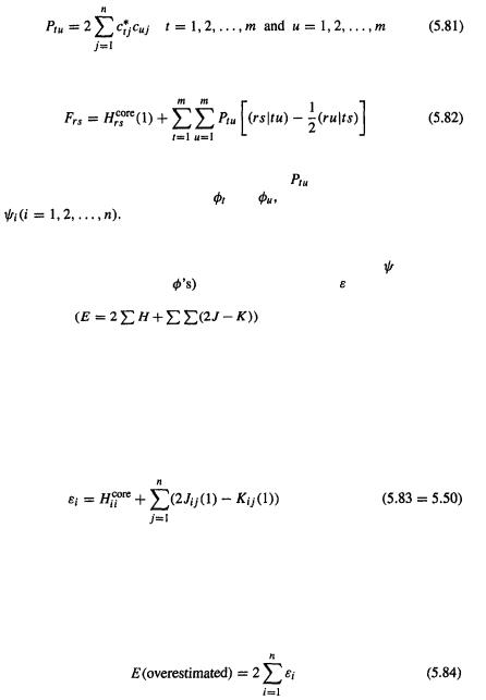
Equation (5.78) is normally modified by subsuming the c’s into  the elements of the density matrix P:
Ab initio calculations 189
where the density matrix elements are
(sometimes P is defined as  From Eqs (5.78) and (5.81):
Equation (5.82), a slight modification of Eq. (5.78), is the key equation in calculating
the ab initio Fock matrix. Each density matrix element |
represents |
the coefficients |
|||
c for a particular pair of basis functions |
and |
summed over |
all the occupied |
||
MO’s |
We use the density matrix here just as a convenient way to |
||||
express the Fock matrix elements, and to formulate the calculation of properties arising from electron distribution (section 5.5.4), although there is far more to the density
matrix concept [21]. Equation (5.82) |
enables the MO wavefunctions |
(which are |
linear combinations of the c’s and |
and their energy levels to be calculated by |
|
iterative diagonalization of the Fock matrix. |
|
|
Equation (5.17) |
gives one expression for the molec- |
|
ular electronic energy E. If we wish to calculate E from the energy levels, we must note that in the HF method E is not simply twice the sum of the energies of the n occupied energy levels, i.e. it is not the sum of the one-electron energies (as we take it to be in the simple and extended Hückel methods). This is because the MO energy level value  represents the energy of one electron subject to interaction with all the other electrons.
The energy of an electron is thus its kinetic energy plus its electron–nuclear attractive potential energy  plus, courtesy of the J and K integrals (section 5.2.3.5 and Eqs (5.48)–(5.50 = 5.83)), the potential energy from repulsion of all the other electrons:
If we add the energies of electrons 1 and 2, say, we are adding, besides the kinetic energies of these electrons, the repulsion energy of electron 1 on electron 2,3,4,..., and the repulsion energy of electron 2 on electron 1, 3,4,... – in other words, we are counting each repulsion twice. The simple sum thus represents properly the total kinetic and electron–nuclear attraction potential energy, but overcounts the electron–electron repulsion potential energy (recall that we are working with electrons and thus
  filled MOs):
Note that we cannot just take half of this simple sum, because only the electron–electron energy terms, not all the terms, have been doubly-counted. The solution is to subtract from  the superfluous repulsion energy; from our discussion of Eq. (5.50) in section 5.2.3.5 we saw that the sum
  over n represents the repulsion energy
190 Computational Chemistry
of one electron interacting with all the other electrons, so to remove the superfluous
interactions we subtract |
the sum over n of the repulsion energy sum, |
to get [13] |
|
 is the HF electronic energy: the sum of one-electron energies corrected (within the average-field HF approximation) for electron–electron repulsion. We can get rid of the integrals J and K over
  and obtain an equation for
  in terms of c’s and
  From (5.83),
and from this and (5.85) we get
From the definition of  in Eqs (5.49) and (5.50), i.e. from
and the LCAO expansion (5.52)
we get from Eq. (5.86)
Using Eq. (5.81), Eq. (5.89) can be written in terms of the density matrix elements P:
This is the key equation for calculating the HF electronic energy of a molecule. It can be used when self-consistency has been reached, or after each SCF cycle employing the  and
and  yielded by that particular iteration, and
  which latter does not change from iteration to iteration, since it is composed only of the fixed basis functions and an operator which does notcontain
 or
or  from Eqs (5.64=5.19) and (5.79)
Ab initio calculations 191
 does not change because the SCF procedure refines the electron–electron repulsion (till the field each electron feels is “consistent” with the previous one), but
  in contrast represents only the contribution to the kinetic energy plus electron-nucleus attraction of the electron density associated with each pair of basisfunctions
 and
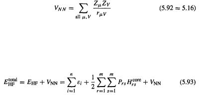
and  Equation (5.90) gives the HF electronic energy of the molecule or atom – the energy of the electrons due to their motion (their kinetic energy) plus their energy due to electron–nucleus attraction and (within the HF approximation) to electron–electron repulsion (their potential energy). The total energy of the molecule, however, involves not just the electrons but also the nuclei, which contribute potential energy due to internuclear repulsion and kinetic energy due to nuclear motion. This motion persists even at 0 K, because the molecule vibrates even at this temperature; this unavoidable vibrational energy is called the zero-point vibrational energy or zero-point energy (ZPVE or ZPE; section 2.5, Fig. 2.20 and associated discussion). Calculation of the internuclear repulsion energy is trivial, as this is just the sum of all coulombic repulsions between
the nuclei:
Calculation of the ZPE is more involved; it requires calculating the frequencies (i.e. the normal-mode vibrations – section 2.5) and summing the energies of each mode [22] (all this is done by standard programs, which print out the ZPE after the frequencies). Adding the HF electronic energy and the internuclear repulsion gives what we might call  the total “frozen-nuclei” (no ZPE) energy:
from (5.90) and (5.92).  the energy usually displayed at the end of a HF calculation is, in ordinary parlance, “the HF energy”. An aggregate of such energies, plotted against various geometries, represents an HF Born–Oppenheimer PES (section 2.3). The zero of energy for the Schrödinger equation for an atom or molecule is normally taken as the energy of the electrons and nuclei at rest at infinite separation. The HF energy (any ab initio energy, in fact) of a species is thus relative to the energy of the electrons and nuclei at rest at infinite separation, i.e. it is the negative of the minimum energy required to break up the molecule or atom and separate the electrons and nuclei to infinity. We are normally interested in relative energies, differences in absolute ab initio energies. Ab initio energies are discussed in section 5.5.2.
In a geometry optimization (section 2.4) a series of single-point calculations (calculations at a single point on the potential energy surface, i.e. at a single geometry) is done, each of which requires the calculation of and the geometry is changed systematically until a stationary point is reached (one where the potential energy surface is flat; ideally
  should fall monotonically in the case of optimization to a minimum). The ZPE calculation, which is valid only for a stationary point on the potential energy surface (section 2.5; discussion in connection with Fig. 2.19), can be used to correct
 of the optimized structure for vibrational energy; adding the ZPE gives the total
192 Computational Chemistry
internal energy of the molecule at 0 K, which we could call 
The relative energies of isomers may be calculated by comparing  but for accurate work the ZPE should be taken into account, even though the required frequency calculations usually take considerably longer than the geometry optimization (sometimes five to ten times as long – see section 5.3.3, Table 5.3). Fortunately, it is valid to correct
 with a ZPE from a lower-level optimization-plus-frequency job (not a lower-level frequency job on the higher-level geometry). Figure 2.19 in section 2.5 compares energies for the species in the isomerization of HNC to HCN. The relative energies with/without the ZPE correction for HCN, transition state, and HNC are 0/0, 202/219, and
  The ZPE’s of isomers tend to be roughly equal and so to cancel when relative energies are calculated (less so where transition states are involved), but, as implied above, in accurate work it is usual to compare the ZPE-corrected energies
5.2.3.6e Using the Roothaan–Hall equations to do ab initio calculations – an example
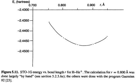
The application of the HF method to an actual calculation will now be illustrated in detail with protonated helium, the simplest closed-shell heteronuclear molecule. This species was also used to illustrate the details of the EHM in section 4.4. 1b. In this simple example all the steps were done with a pocket calculator, except for the evaluation of the integrals (this was done with the ab initio program Gaussian 92 [23]) and the matrix multiplication and diagonalization steps (done with the program Mathcad [24]).
Step 1 Specifying the geometry, basis set and MO orbital occupancy
We start by specifying a geometry and a basis set. We will use same geometry as with the EHM, 0.800 Å, i.e. 1.5117 a.u. (bohr). In ab initio calculations on molecules, the basis functions are almost always Gaussian functions (basis functions are discussed in section 5.3). Gaussian functions differ from the Slater functions we used in the EHM in chapter 4 in that the exponent involves the square of the distance of the electron from the point (usually an atomic nucleus) on which the function is centered:
An s-type Slater function
An s-type Gaussian function
In ab initio calculations the mathematically more tractable Gaussians are used to approximate the physically more realistic Slater functions (see section 5.3). We use here the simplest possible Gaussian basis set: a 1s atomic orbital on each of the two atoms, each 1s orbital being approximated by one Gaussian function. This is called an STO-1G basis set, meaning Slater-type orbitals-one Gaussian, because we are approximating a Slater-type 1s orbital with a Gaussian function. The best STO-1G approximations to

Ab initio calculations 193
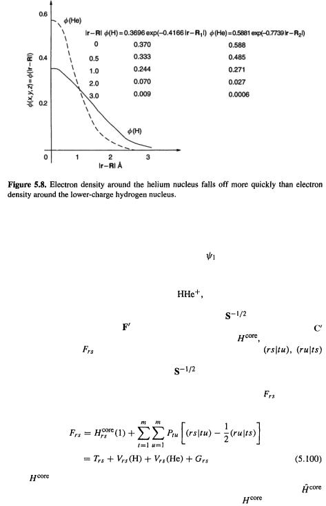
the hydrogen and helium 1s orbitals in a molecular environment [25] are
where  is the distance of the electron in
 is a one-electron function) from nucleus i on which
  is centered (Fig. 5.7). The larger constant in the helium exponent as compared to that of hydrogen (0.7739 vs. 0.4166) reflects the intuitively reasonable
fact that since an electron in |
is bound more tightly to its doubly-charged nucleus |
|
than is an electron in |
is to its singly-charged nucleus, electron density around the |
|
helium nucleus falls off more quickly with distance than does that around the hydrogen
nucleus (Fig. 5.8). |
|
|
We have a geometry and a basis set, and wish to do an SCF calculation on |
with |
|
both electrons in the lowest MO, |
i.e. on the singlet ground state. In general, SCF |
|
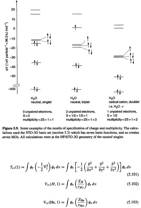
calculations proceed from specification of geometry, basis set, charge and multiplicity. The multiplicity is a way of specifying the number of unpaired electrons:
194 Computational Chemistry
where s = total number of unpaired electron spins (each electron has a spin of  taking each unpaired spin as
  Figure 5.9 shows some examples of the specification of charge and multiplicity. By default an SCF calculation is performed on the ground state of specified multiplicity, i.e. the MO’s are filled from up to give the lowest-energy state of that multiplicity.
Step 2 Calculating the integrals |
|
Having specified a HF calculation on singlet |
with H–He = 0.800Å (1.5117 |
bohr), using an STO-1G basis set, the most straightforward way to proceed is to now
calculate all the integrals, and the orthogonalizing matrix |
that will be used to |
||
transform the Fock matrix Fto |
and to convert the transformed coefficient matrix |
||
to C (Eqs (5.67)–(5.70)). The integrals are those required for |
the one-electron |
||
part of the elements |
of F, and the two-electron repulsion integrals |
||
(Eq. (5.82)), as well as the overlap integrals, which are needed to calculate the overlap
matrix S and thus the orthogonalizing matrix |
(Eq. (5.67)). |
Efficient methods have been developed for calculating these integrals [26] and their
values will simply be given here. For our calculation the elements |
of the Fock |
matrix (Eq. (5.82)) are conveniently written as: |
|
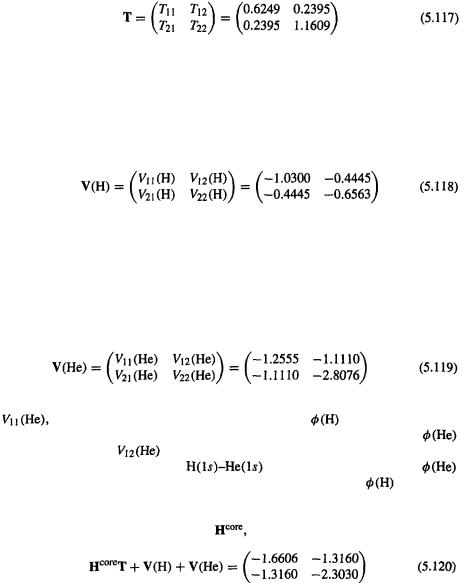
Here |
(1) has been dissected into a kinetic energy integral T and two poten- |
|
tial energy integrals, V (H) and V (He). From the definition of the operator |
||
(Eq. (5.64)) and the Roothaan–Hall expression for the integral |
(Eq. (5.79)) we |
|
Ab initio calculations 195
see that (the (1) emphasizes that these integrals involve the coordinates of only one electron):
and
In Eq. (5.102) the variable is the distance of the electron (“electron 1” – see the discussion in connection with Eqs (5.18) and (5.19)) from the hydrogen nucleus, and in Eq. (5.103)
196 Computational Chemistry |
|
|
the variable is the distance of the electron from the helium nucleus; |
and |
are 1 |
and 2, respectively.
From Eq. (5.100) the two-electron contribution to the each Fock matrix element is
Each element |
is calculated from a density matrix |
element |
(Eqs (5.80) |
|
and (5.81)) and two two-electron integrals |
and |
(Eqs (5.73) and (5.77)). |
||
The required one-electron integrals for calculating the Fock matrix F are
To see which two-electron integrals are needed we evaluate the summation in Eq. (5.104) for each of the matrix elements 
Ab initio calculations |
197 |
Each element of the electron repulsion matrix G has eight two-electron repulsion integrals, and of these 32 there appear to be 14 different ones:
from |
(11|11), (11|12), (12|11), (11|21), (11|22), (12|21) |
new with |
(12|12), (12|22) |
new with |
(22|11), (21|12), (22|12), (22|21), (21|22), (22|22) |
However, examination of Eq. (5.73) shows that many of these are the same. It is easy to see that if the basis functions are real (as is almost always the case) then
Taking this into account, there are only six unique two-electron repulsion integrals, whose values are:
(11|11) = 0.7283 |
(21|21) = 0.2192 |
|
(21|11) = 0.3418 |
(22|21) = 0.4368 |
(5.110) |
(22|11) = 0.5850 |
(22|22) = 0.9927 |
|
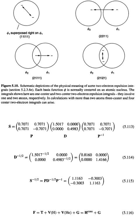
The integrals (11|11) and (22|22) represent repulsion between two electrons both in
the same orbital |
or |
respectively), while (22|11) represents repulsion between |
||
an electron in |
and one in |
(21|11) could be regarded as representing the repulsion |
||
between an electron associated with |
and and one confined to |
and analogously |
||
for (22|21), while (21|21) can be thought of as the repulsion between two electrons
both of which are associated with |
and |
(Fig. 5.10). Note that in the T and V terms |
||
of the Fock matrix elements, the operator in the integrals is |
and |
|||
or |
while in the G terms it is |
(Eqs (5.101)–(5.103) |
and (5.73)). The |
|
overlap integrals are |
|
|
|
|
and the overlap matrix is
Step 3 Calculating the orthogonalizing matrix
Calculating the orthogonalizing matrix |
(see Eqs (5.67)–(5.69) and the discussion |
referred to in chapter 4): |
|
198 Computational Chemistry
Diagonalizing S:
Calculating 
Calculating 
Step 4 Calculating the Fock matrix
(a) The one-electron matrices
From Eq. (5.100)
Ab initio calculations 199
The one-electron matrices T, V(H) and V(He) (i.e.  follow immediately from the one-electron integrals. The kinetic energy matrix is
 is smaller than
  as the kinetic energy of an electron in
  is smaller than that of an electron in
  this is expected since the larger charge on the helium nucleus results in a larger kinetic energy for an electron in its
  orbital than for an electron in the hydrogen
  orbital–classically speaking, the electron must move faster to stay in orbit around the stronger-pulling He nucleus.
  can be regarded as the kinetic energy of an electron in the
 overlap region.
The hydrogen potential energy matrix is
All the V(H) values represent the attraction of an electron to the hydrogen nucleus.  is the potential energy due to attraction of an electron in
  to the hydrogen nucleus, and
  is the potential energy due to attraction of an electron in
  to the hydrogen nucleus. As expected, an electron in
  is attracted to the H nucleus more strongly (the potential energy is more negative) than is an electron in
 can be regarded as the potential energy of attraction to the hydrogen nucleus of an electron in the
  overlap region.
The helium potential energy matrix is
All the V(He) values represent the attraction of an electron to the helium nucleus.
the potential energy of attraction of an electron in |
to the helium nucleus, |
|||
is of course less negative than the potential energy of attraction of an electron in |
||||
to this same nucleus. |
can be taken as the potential energy of attraction to the |
|||
helium nucleus of an electron in the |
overlap region. An electron in |
|||
is attracted to the helium nucleus more strongly than an electron in |
is attracted |
|||
to the hydrogen nucleus (–2.8076 in V(He) cf. –1.0300 in V(H)), due to the greater
nuclear charge of helium. |
|
The total one-electron energy matrix, |
is |
This matrix represents the 1-electron energy (the energy the electron would have if interelectronic repulsion did not exist) of an electron in  at the specified geometry, for this STO-1G basis set. The (1,1), (2,2) and (1,2) terms represent, ignoring electron–electron repulsion, the energy of an electron in
  and the
  overlap region, respectively; the values are the net result of the various kinetic energy and potential energy terms discussed above.
200 Computational Chemistry
(b) The two-electron matrix
The two-electron matrix G, the electron repulsion matrix (Eq. (5.111)), is calculated from the two-electron integrals and the density matrix elements (Eq. (5.104)). This is intuitively plausible since each two-electron integral describes one interelectronic repulsion in terms of basis functions (Fig. 5.10) while each density matrix element represents (see section 5.4.3) the electron density on (the diagonal elements of P in Eq. (5.80)) or between (the off-diagonal elements of P) basis functions. To calculate the matrix elements  (Eqs (5.106)–(5.108)) we need the appropriate integrals (Eqs (5.110) and density matrix elements. These latter are calculated from
Each  involves the sum over the occupied MO’s
  we are dealing with a closed-shell ground-state molecule with
  electrons) of the products of the coefficients of the basis functions
  and
and  As pointed out in section 5.2.3.6b the HF procedure is usually started with an “initial guess” at the coefficients. We can use as our guess the extended Hückel coefficients we obtained for
  with this same geometry (section 4.4. 1b); we need the c’s only for the occupied MO’s:
(Usually we need more c’s than the small basis set of an extended Hückel or other semiempirical calculation supplies; a projected semiempirical wavefunction is then used, with the missing c’s extrapolated from the available ones.) Using these c’s and Eq. (5.121) we calculate the initial-guess P’s for Eqs. (5.106)–(5.108); since there is only one occupied MO  in Eq. 121) the summation has only one term:
G may now be calculated. From Eqs (5.106)–(5.108), using the above values of P and the integrals of Eq. (5.110), and recalling that integrals like (11|12) and (21|11) are equal (Eq. (5.109) we get:
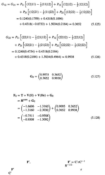
Ab initio calculations 201
From the G values based on the initial guess c’s the initial-guess electron repulsion matrix is
The initial-guess Fock matrix is (Eqs (5.116), (5.120) and (5.127))
The zero subscripts in Eqs (5.127) and (5.128) emphasize that the initial-guess c’s, with no iterative refinement, were used to calculate G; in the subsequent iterations of the SCF procedure  will remain constant while G will be refined as the c’s, and thus the P’s, change from SCF cycle to cycle. The change in the electron repulsion matrix G corresponds to that in the molecular wavefunction as the c’s change (recall the LCAO expansion); it is the wavefunction (squared) which represents the time-averaged electron distribution and thus the electron/charge cloud repulsion (sections 5.2.3.2, 5.2.3.5 and 5.2.3.6b).
Step 5 Transforming F to |
the Fock matrix that satisfies |
|
|
As in section 4.4. 1b, we use the orthogonalizing matrix |
(step 3) to transform |
||
F to a matrix |
which when diagonalized gives the energy levels and a coeffi- |
||
cient matrix |
which is subsequently transformed to the matrix C of the desired c’s |
||
202 Computational Chemistry
(see section 5.2.3.6b):
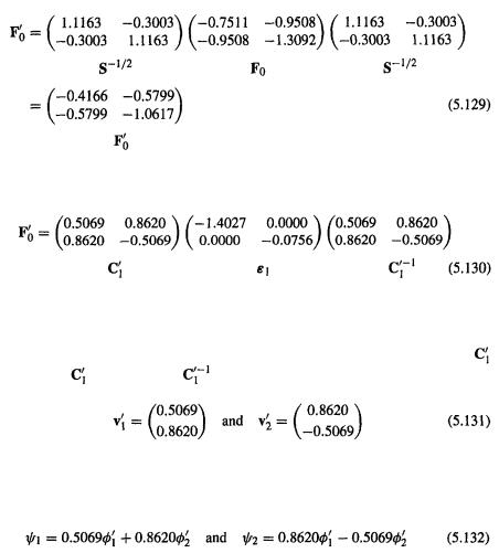
Step 6 Diagonalizing  to obtain the energy level matrix
 and a coefficient matrix
The energy levels (the eigenvalues of  ) from this first SCF cycle are – 1.4027 and
–0.0756 h (h = hartrees, the unit of energy in atomic units), corresponding to the occupied MO  and the unoccupied MO
  The MO coefficients (the eigenvectors of
  of
of and
and  for the transformed, orthonormal basis functions, are, from
(actually here |
and its inverse, |
are the same): |
 is the first column of
 and
and  is the second column of
 These coefficients are the weighting factors that with the transformed, orthonormal basis functions give the MO’s:
where and
and  are linear combinations of our original basis functions
  and
and  The original basis functions
 were centered on atomic nuclei and were normalized but not orthogonal (section 4.3.3), while the transformed basis functions
  are delocalized over the molecule and are orthonormal (section 4.4.1a)). Note that the sum of the squares of the coefficients of
  and
and  is unity, as must be the case if the basis functions are orthonormal (section 4.3.6). In the next step
 is transformed to obtain the coefficients of the original basis functions
  in the MO’s. We want the MOs in terms of the original, atom-centered basis functions (roughly, atomic orbitals – section 5.3) because such MOs are easier to interpret.
Step 7 Transforming  to C, the coefficient matrix of the original, nonorthogonal basis functions.
Ab initio calculations 203
As in section 4.4. 1b, we use the orthogonalizing matrix  to transform
 to C:
to C:
This completes the first SCF cycle. We now have the first set of MO energy levels and basis function coefficients:
From Eq. (5.130):
From Eq (5.133) (cf. Eq (5.132)):
Note that the sum of the squares of the coefficients of  and
and  is not unity, since these atom-centered functions are not orthogonal (contrast the simple Hückel method, section 4.3.4).
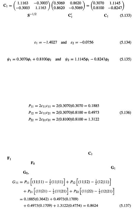
Step 8 Comparing the density matrix from the latest c’s with the previous density matrix to see ifthe SCF procedure has converged
The density matrix elements based on the c’s of  (Eq. (5.133) can be compared with those (Eq. (5.123)) based on the initial guess:
Suppose our convergence criterion was that the elements of P must agree with those of the previous P matrix to within 1 part in 1000. Comparing Eqs (5.136) with (5.123) we see that this has not been achieved: even the smallest change is |(1.312 – 1.503)/1.503| = 0.127, far above the required 0.001. Therefore another SCF cycle is needed.
Step 9 Beginning the second SCF cycle: using the c’s of |
to calculate a new Fock |
|||
matrix |
(cf. Step 4, (b)) |
|
|
|
The first Fock matrix |
used c’s from our initial guess (Step 4, (b)). An improved F |
|||
may now be calculated using the c’s from the first SCF cycle. Calculating |
as we did |
|||
in Step 4, (b) for |
but using the new P’s: |
|
|
|
204 Computational Chemistry
From the G values based on the first-cycle c’s the electron repulsion matrix is
and the Fock matrix from this is
Step 10 Transforming to
to (cf. Step 5)
Step 11 Diagonalizing  to obtain the energy levels ε and a coefficient matrix
  (cf. Step 6)
Ab initio calculations 205
The energy levels from this second SCF cycle are –1.4447 and –0.1062h. To get the MO coefficients corresponding to these MO energy levels in terms of the original basis functions  and
and  we now transform
  to
to 
Step 12 Transforming to
to  (cf. Step 7)
This completes the second SCF cycle. We now have the MO energy levels and basis function coefficients:
From Eq. (5.143):
From Eq. (5.144):
Step 13 Comparing the density matrix from the latest c’s with the previous density matrix to see if the SCF procedure has converged
The density matrix elements based on the c’s of  are
are
Comparing the above with (5.136) we see that convergence to within our 1-part-in- 1000 criterion has not occurred: the largest change in the density matrix is |(0.1996 – 0.1885)/0.1885| = 0.059, which is above 0.001, so the SCF procedure is repeated.
Three more SCF cycles were carried out; the results of the “zeroth cycle” (the initial guess) and the five cycles are summarized in Table 5.1. Only with the fifth cycle has convergence been achieved, i.e. have the changes in all the density matrix elements fallen below 1 part in 1000 (the largest change is in  | (0.2020 – 0.2019)/0.2019 = 0.0005 < 0.001). In actual practice, a convergence criterion of from about 1 part in
  to 1 in
  is used, depending on the program and the particular kind of calculation. The coefficients and the density matrix elements change smoothly, although the energy levels and
  show some oscillation. To reduce the number of steps needed to achieve convergence, programs sometimes extrapolate the density matrix, i.e. estimate the final P values and use these estimates to initiate the final few SCF cycles.
Often the main result from a HF (i.e. an SCF) calculation is the energy of the molecule (the calculation of energy may be subsumed into a geometry optimization, which is really the task of finding the minimum-energy geometry). The STO-1G energy of
with an internuclear distance of 0.800 Å may be calculated from our results: the electronic energy is

206 Computational Chemistry
Ab initio calculations 207
the internuclear repulsion energy is
and the total internal energy of the molecule at 0 K (except for ZPE – section 5.2.3.6d) is
 which is what is normally meant by the HF energy, is printed by the program at the end of a single-point calculation or a geometry optimization, or by some programs at the end of each step of a geometry optimization.
Using the energy levels and density matrix elements from the first cycle (Table 5.1), with the elements from Eq. (5.120), Eq. (5.147) gives for the electronic energy
From Eq. (5.148) the internuclear repulsion energy is
and from Eq. (5.149) the total HF energy is
The HF energies for the five SCF cycles are given in Table 5.1.
Instead of starting with eigenvectors from a non-SCF method like the extended Hückel method, as was done in this illustrative procedure, an SCF calculation is occasionally initiated by taking  as the Fock matrix, that is, by initially ignoring electron–electron repulsion, setting equal to zero the second term in Eq. (5.82), or G in Eq. (5.100), whereupon
  becomes
  This is usually a poor initial guess, but is occasionally useful. You are urged to work your way through several SCF cycles starting with this Fock matrix; this tedious calculation will help you to appreciate the power
208 Computational Chemistry
and utility of modern electronic computers and may enhance your respect for those who pioneered complex numerical calculations when the only arithmetical aids were mathematical tables and mechanical calculators (mechanical calculators were machines with rotating wheels, operated by hand-power or electricity. There were also, in astronomy at least, armies of women arithmeticians called computers – the original meaning of the word).
If we calculate the electronic energy simply as twice the sum of the energies of the occupied MO orbitals, as with the SHM and EHM, we get a much higher value than from the correct procedure (Eq. (5.147)); with a 0.800 Å bond length and the converged results this naive electronic energy is 2(–1.4470) h = –2.8940 h, while the correct electronic energy (not given in Table 5.1 – the HF energies there are electronic plus internuclear repulsion) is –3.7668 h, i.e. 30 percent lower when we correct for the fact that simply double-summing the MO energies counts electron repulsion terms twice (section 5.2.3.6d).
A geometry optimization for  can be done by calculating the Hartree-Fock energy (electronic plus internuclear) at different bond lengths to get the minimumenergy geometry. The results are shown in Fig. 5.11; the optimized bond length for the STO-1G basis set is ca. 0.86 Å. Note that it is customary to report ab initio energies in hartrees to 5 or 6 decimal places (and bond lengths in Å to 3 decimals); the truncated values used here are appropriate for these illustrative calculations.
Summary of the steps in an SCF calculation using the Roothaan–Hall LCAO expansion of the MO’s
1.Specify a geometry, basis set, and orbital occupancy (this latter is done by specifying the charge and multiplicity, with an electronic ground state being the default).

Ab initio calculations 209
2. Calculate the integrals:  for each nucleus, and the two-electron integrals
  etc. needed for
  as well as the overlap integrals
 for the orthogonalizing matrix derived from S (see step 3). Note: in the direct SCF method (section 5.3) the
two-electron integrals are calculated as needed, rather than all at once.
3.Calculate the orthogonalizing matrix 
(a)diagonalize
(b)Calculate  (take the
  power of the elements of D)
(c)Calculate 
4.Calculate the Fock matrix F
(a) Calculate the one-electron matrix |
using the T and |
Vintegrals from step 2.
(b)The two-electron matrix (the electron repulsion matrix) G: Use an initial guess of the coefficients of the occupied MO’s to calculate initial-guess density matrix elements:
Use the density matrix elements and the two-electron integrals to calculate G:
The Fock matrix is
5.Transform F to  the Fock matrix that satisfies
6.Diagonalize to get energy levels and a
 matrix
7.Transform  to C, the coefficient matrix of the original basis functions
8.Compare the density matrix elements calculated from the C of the previous step with those of the step before that one (and/or use other criteria, e.g. the molecular
energy); if convergence has not been achieved go back to step 4 and calculate a new Fock matrix using the P’s from the latest c’s. If convergence has been achieved, stop.
It should be realized modern ab initio programs do not rigidly follow the basic SCF procedure described in this section. To speed up calculation they employ a variety of mathematical tricks. Among these are: the use of symmetry to avoid duplicate calculation of identical integrals; testing two-electron integrals quickly to see if they are