268 Computational Chemistry

5.5.2.2Energies: calculating quantities relevant to thermodynamics and to kinetics

5.5.2.2a Thermodynamics; “direct” methods, isodesmic reactions

Here we are concerned with the relative energies of species other than transition states. Such molecules are sometimes called “stable species,” even if they are not at all stable in the usual sense, to distinguish them from transition states, which exist only for an instant on the way from reactants to products, A “stable species,” in contrast, sits in a potential energy well and survives at least a few molecular vibrations The very useful book by Hehre [32] contains a wealth of information on computational and experimental results concerning thermodynamic quantities.

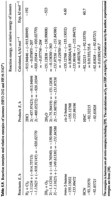
The ab initio reaction energy that is most commonly calculated is simply the difference in ZPE-corrected energies, which is the reaction enthalpy change at 0 K (Eq. (5.176)). This provides an easily-obtained indication of whether a reaction is likely to be exothermic or endothermic, or of the relative stabilities of isomers. Table 5.9 illustrates this procedure. The results are only semiquantitatively correct, and the HF/6-31G* method is not necessarily better here than the HF/3-21G. In fact, it has been documented by extensive calculations that such HF/3-21G and HF/6-31G* energy differences generally give only a rough indication of energy changes. Much better results are obtained from MP2/6-31G* calculations on MP2/6-31G*, HF/3-21G* or even semiempirical AM1 geometries, and it is well worth consulting the book by Hehre for details [108].

To get the best results from relatively low-level calculations, one can utilize isodesmic reactions (Greek: “same bond,” i.e. similar bonding on both sides of the equation). These are reactions in which the number of each kind of bond and each kind of lone pair is conserved. For example,

and

are isodesmic reactions; the first one has on each side 6 N–H bonds, one C–N bond and one nitrogen lone pair, and the second has on each side 6 C–H and 2 C–F bonds. The reaction

is, strictly speaking, not isodesmic, since although it has the same number ofbonds, even the same number of single bonds, on both sides, there are 6 C–H, one C–C, and 2 H–H bonds on one side and 8 C–H bonds on the other. Note that an isodesmic reaction does not have to be experimentally realizable: it is an artifice to obtain a reasonably accurate energy difference by ensuring that as far as possible errors cancel. This will happen to the extent that particular errors are associated with particular structural features; electron correlation effects are thought to be especially important in calculating energy differences, and such effects tend to cancel when the number of electron pairs of each kind is conserved.

Reactions like (5.182) give fairly good quantitative results for the proton affinities (essentially, the basicity) of nitrogen bases [109], byusing to deprotonate a series

Ab initio calculations 269

270 Computational Chemistry

oftheconjugate acids. Isodesmic processes like (5.183) have been used to reveal the nature and amount of interaction between groups X and Y on an carbon [110]. IfX and Y interact in a stabilizing way, then separating them should be reflected in an endothermic reaction, and conversely mutually destabilizing groups should give an exothermic reaction. For reaction (5.183) at the 3-21G level the product energies minus the reactant energies are i.e. the reaction is endothermic by while for the corresponding reaction the reaction energy is which indicates a qualitatively different mutual interaction between two fluorines, as compared to two chlorines, on the same carbon (actually, a bigger basis set indicates that the Cl/Cl interaction in is about zero). Another application of isodesmic reactions has been to estimating aromatic character [111].

There is no unique isodesmic reaction for a particular problem. For example, to compare the ring strain in oxacyclopropane (oxirane, ethylene oxide) with that in cyclopropane, one might calculate the reaction energy of the oxygen exchange reaction (remember that isodesmic reactions do not have to be experimentally achievable):

Here the equilibrium should favor the less-strained ring. Alternatively, one might compare the reaction energies of the two cleavage reactions:

Here, the reaction that forms the less-strained ring should be the less endothermic (or the more exothermic, if the reactions turn out to be exothermic).

Let us calculate the reaction energies for the three reactions. For (5.185), the HF/6-31G* (including ZPE) energies are

E(pdts) – E(reactants)

The reaction is calculated to be exothermic by and the simple interpretation is that cyclopropane is more strained than oxacyclopropane by To compare oxacyclopropane and cyclopropane using (5.186) and (5.187), we do need not calculate the energies of and since these will cancel out:

Ab initio calculations 271

and for (187):

Reaction (5.187) is more endothermic than reaction (5.186)by 1.18152 – 1.17357 h = 0.00795 h = indicating that cyclopropane is more strained than oxacyclopropane by this amount [112]. The agreement between the two approaches is not coincidental, since the cancellation of the methane and the ethane energies makes these two conceptually different approaches mathematically identical. Note, however, that for any isodesmic reaction we can always write some non-equivalent (unlike the case of (5.185) vs. (5.186)/(5.187)) isodesmic process to get the desired quantity. Also, different isodesmic reactions will give somewhat different results; this is essentially because the “reagents” of one reaction will not be calculated to exactly the same degree of accuracy as those of another reaction.

As we saw in section 5.4.1, calculation of homolytic cleavage energies by simply subtracting HF energies gives very poor results. Let us calculate a homolytic bond dissociation energy by an isodesmic-type approach. The idea is to combine the desired homolytic reaction with one of known (either from experiment or from as high-level calculation) energy in a reaction which, although not strictly isodesmic, conserves the number ofsingle, double, etc. bonds and the numberofunpaired electrons. Forexample,

Here E(C–C) and E(C–O) are homolytic dissociation energies(bond energies) and E(iso) is the energy of the isodesmic-type reaction shown. This reaction is not strictly isodesmic, since a C–C bond is replaced by a C–O bond, but it does have the same number of unpaired electrons(one) on each side, so net correlation effects should be much less than for a reaction in which two unpaired electrons are created from a bond. A reaction in which the number of unpaired electrons is conserved is called an isogyric(Greek, “same spin”) reaction. Since the overall energy change in a process is independent of the path connecting the initial and final states [113] we write

i.e.

E(C–C) must be known, and E(iso) is to be obtained by calculation. Taking an experimental value of for the bond energy of the ethane C–C bond [61], and