Ab initio calculations 297

requires a knowledge of the shapes of the drug and of the active site [82]). The relative energies of molecular species is fundamental to a knowledge of their kinetic and thermodynamic behaviour, and this can be important in attempts to synthesize them. The vibrational frequencies of a molecule, provide information about the electronic nature of its bonds, and prediction of the spectra represented by these frequencies may be useful to experimentalists.

A fourth important characteristic of a molecule is the distribution ofelectron density in it. Calculation of the electron density distribution enables one to predict the dipole moment, the charge distribution, the bond orders, and the shapes of various molecular orbitals.

Dipole moments

The dipole moment [ 161 ] of a system of two charges Q and – Q separated by a distance is, by definition, the vector Qr ; the direction of the vector is officially from – Q toward +Q, but chemists usually assign a molecular or bond dipole (see below) the direction from the positive end of the bond or molecule to the negative (Fig. 5.37(a)). The dipole moment of a collection of charges with corresponding

position vectors(Fig. 5.37(b)) is

and the so the dipole moment of a molecule is seen to arise from the charges and positions of its component electrons and nuclei. The dipole moment of a molecule is an experimental observable [162], with which we can compare calculated moments. It is often convenient to think of the molecular dipole moment as the vector sum of bond moments (Fig. 5.37(c)). Two points should be noted: we are discussing an average dipole moment, because electron and nuclear motions will cause the dipole moment to fluctuate, so that even a spherical atom can have temporary nonzero dipole moments. Another point is that we usually consider the dipole moments of neutral molecules only, not of ions; this is because the dipole moment of a charged species is not unique, but depends on the choice of the point in the coordinate system from which the position vectors are measured.

Let us look at the calculation of the dipole moment within the HF approximation. The quantum mechanical analogue of Eq. (5.200) for the electrons in a molecule is

Here the summation of charges times position vectors is replaced by the integral over thetotalwavefunction (the square of the wavefunction is a measure of charge) of the dipole moment operator (the summation over all electrons of the product of an electronic charge and the position vectors of the electrons). To perform an ab initio calculation of the dipole moment of a molecule we want an expression for the moment in terms of the basis functionstheir coefficientsand the geometry (for a molecule of specified charge and multiplicity these are the only “variables” in an ab initio calculation). The HF

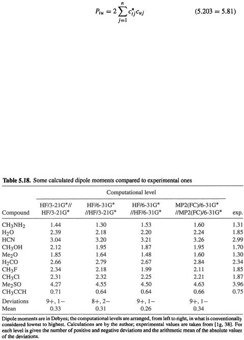
Ab initio calculations 299

Here the first term refers to the nuclear charges and position vectors and the second term (the double summation) refers to the electrons. = the density matrix elements (sections 5.2.3.6d and 5.2.3.6e), cf.:

The P summation is over the occupied orbitals ( j = 1,2,..., n; we are considering closed-shell systems, so there are 2n electrons) and the double summation is over the m basis functions. The operator r is the electronic position vector.

How good are ab initio dipole moments? Hehre’s extensive survey of practical ab initio methods [32] indicates that fairly good results are given by HF/6-31G*//HF/6-31G* (dipole moment from a HF/6-31G* calculation on a HF/6-31G* geometry) calculations, and that MP2/6-31G*//MP2/6-31G* calculations are usually not much better. Some calculated and experimental dipole moments are compared in Table 5.18. These results, which are quite typical, indicate that calculated values tend to be about 0.0–0.5 D higher than experimental, with a mean deviation of about 0.3 D; negative deviations are rare. HF/3-21G//HF/3-21G (the lowest ab initio level likely to be used) calculations may show the largest deviations. Single-point HF/6-31G* calculations on HF/3-21G geometries appear to give results about as good as (or better than? Note and [32], pp. 76, 77) those from MP2(FC)/6-31G*//MP2(FC)/6-31G* calculations. As is the case for other properties, 3-21G calculations of dipole moments on molecules with atoms beyond neon require

300 Computational Chemistry

polarization functions for reasonable results (the 3-21G(*) basis; [32], pp. 23–30). The 3-21G* calculations in Table 5.18 show a mean deviation 0.33; the HF/6-31G* calculations are only slightly better (mean deviation 0.26) and the MP2/6-31G* calculations appear to be, if anything, slightly worse (mean error 0.34). If high-accuracy calculated dipole moments (0.1 D or better) are needed, high-level correlation and large basis sets must be used; such calculations may be needed to reproduce the magnitude and even the direction of small dipole moments, e.g. in carbon monoxide [163].

Charges and bond orders

Chemists make extensive use of the idea that the atoms in a molecule can be assigned electrical charges. Thus in a water molecule each hydrogen atom is considered to have an equal, positive, charge, and the oxygen atom to have a negative charge (equal in magnitude to the sum of the hydrogen charges). This concept is clearly related to the dipole moment: in a diatomic (for simplicity) molecule one expects the negative end of the dipole vector to point toward the atom assigned the negative charge. However, there are two problems with the concept: first, the charge on an atom in a molecule, unlike the dipole moment of a molecule, cannot be measured (it is not an observable). Second, there is no unique, correct theoretical method for calculating the charge on an atom in a molecule.

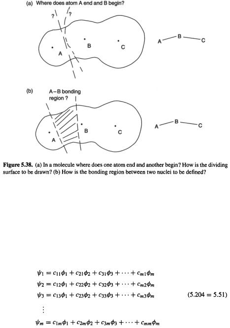
Both the measurement and calculational problems arise from the difficulty of defining what we mean by “an atom in a molecule”. Consider the hydrogen chloride molecule. As we move from the hydrogen nucleus to the chlorine nucleus, where does the hydrogen atom end and the chlorine atom begin? If we had a scheme for partitioning the molecule into atoms (Fig. 5.38(a)), the charge on each atom could be defined as the net electric charge within the space of the atom, i.e. the algebraic sum of the electronic and the nuclear charges. The electronic charge in the defined space could be found by integrating the electron density (essentially the square of the wavefunction; only the wavefunction composed of the occupied orbitals need be considered) over that region of space.

Bondorder is a term with conceptual difficulties related to those associated with atom charges. The simplest electronic interpretation of a bond is that it is a pair of electrons shared between two nuclei, somehow [164] holding them together. From this criterion and Lewis structures the C/C bond order in ethane is 1, in ethene 2, and in ethyne 3, in accordance with the classical assignment of a single, a double, and a triple bond, respectively. However, if a bond is a manifestation of the electron density between two

the group might drain electron density away toward the electronegative oxygen. However, an attempt to calculate bond order from electron density (the square of the wavefunction) runs into the problem that in a polyatomic molecule, at any rate, it is not clear how to define precisely the region “between” two atomic nuclei (Fig. 5.38(b)).

Assigning atom charges and bond orders involves calculating the number of electrons “belonging to” an atom or shared “between” two atoms, i.e. the “population” of electrons on or between atoms; hence such calculations are said to involve population analysis. Earlier schemes for population analysis bypassed the problem of defining the space occupied by atoms in molecules, and the space occupied by bonding electrons, by partitioning electron density in a somewhat arbitrary way. The earliest such schemes

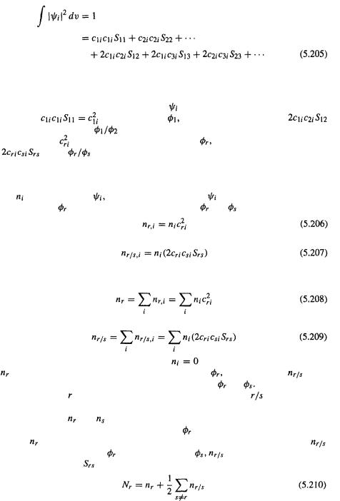
302 Computational Chemistry

over all space gives

The integral equals one because the probability that the electron is somewhere in the MO (which, strictly, extends over all space) is one; the (both the same) overlap integrals are also unity, since the basis functions are normalized (cf. section 4.4.1 b).

(1), the terms sum to one (the “fractions” of the electron must add to one), and (2) it seems reasonable to partition the contribution of electrons to basis functions and overlap regions according to the “electron density sum” in Eq. (5.205). Now if there

and

The total contributions from all the MOs to the electron population in and in the overlap region between and are

and

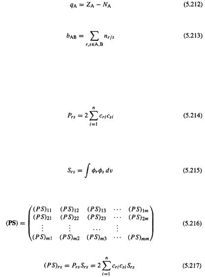
304 Computational Chemistry

This is the sum over all the basis functions on atom A A qualifying the summation means “r belonging to A”) of the gross populations in each (Eq. (5.210); it involves all the basis functions on A and all the overlap regions these functions have with other basis functions We can regard as the total electron population on atom A (within the limits of the Mulliken treatment). The Mulliken charge on atom A, the net charge on A, is then simply the algebraic sum of the charges due to the electrons and the nucleus:

The Mulliken bond order for the bond between atoms A and B is the total population for the A/B overlap region:

The overlap population for basis functions and (Eq. (5.209)) is summed over all the overlaps between basis functions on atoms A and B.

Since the formulas for calculating Mulliken charges and bond orders (Eqs (5.206)- (5.213)) involve summing basis function coefficients and overlap integrals, it is not too surprising that they can be expressed neatly in terms of the density matrix (section 5.2.3.6d) P and the overlap matrix S (section 4.3.3). The elements of the density matrix P are

The matrix element is summed over all filled MOs (from to for the ground electronic state of a 2n-electron closed-shell molecule); an example of the calculation of P was given in section 5.2.3.6e. The elements of the overlap matrix S are simply the overlap integrals:

From Eq. (5.214) it follows that the matrix (PS) obtained by multiplying corresponding elements of P and S,

has elements

Note that (PS) is not the matrix PS obtained by matrix multiplication of P and S; each element of that matrix would result from series multiplication: a row of P times a column of S (section 4.3.3).