50 Computational Chemistry

Setting we find that for this point on the curve i.e.

If we set (from Eq. (3.6)) in Eq. (3.5), we find

i.e.

So can be calculated from the depth of the energy minimum.

In deciding to use equations of the form (3.2)–(3.5) we have decided on a particular MM forcefield. There are many alternative forcefields. For example, we might have chosen to approximate by the sum of a quadratic and a cubic term:

This gives a somewhat more accurate representation of the variation of energy with length. Again, we might have represented the nonbonded interaction energy by a more complicated expression than the simple 12-6 potential of Eq. (3.5) (which is by no means the best form for nonbonded repulsions). Such changes would represent changes in the forcefield.

3.2.2 Parameterizing a forcefield

We can now consider putting actual numbers, etc., into Eqs (3.2)– (3.5), to give expressions that we can actually use. The process of finding these numbers is called parameterizing (or parametrizing) the forcefield. The set of molecules used for parameterization, perhaps 100 for a good forcefield, is called the training set. In the purely illustrative example below we use just ethane, methane and butane.

Parameterizing the bond stretching term. A forcefield can be parameterized by reference to experiment (empirical parameterization) or by getting the numbers from high-level ab initio or density functional calculations, or by a combination of both approaches. For the bond stretching term of Eq. (3.2) we need and Experimentally, could be obtained from IR spectra, as the stretching frequency of a bond depends on the force constant (and the masses of the atoms involved) [8], and could be derived from X-ray diffraction, electron diffraction, or microwave spectroscopy [9].

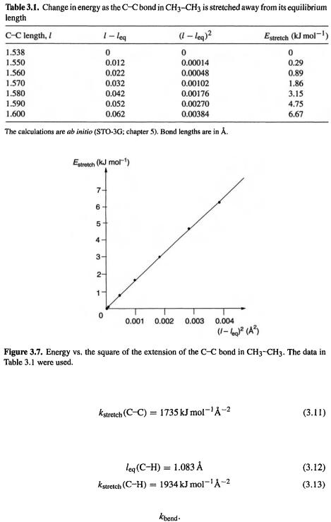
Let us find for the C/C bond of ethane by ab initio (chapter 5) calculations. Normally high-level ab initio calculations would be used to parameterize a forcefield, but for illustrative purposes we can use the low-level but fast STO-3G method [10]. Eq. (3.2) shows that a plot of against should be linear with a slope of Table 3.1 and Fig. 3.7 show the variation of the energy of ethane with stretching of the C/C bond, as calculated by the ab initio STO-3G method. The equilibrium bond

length has been taken as the STO-3G length:

52 Computational Chemistry

the H–C–C angle in ethane we get (cf. Table 3.1 and Fig. 3.7)

Calculations on staggered butane gave for the C–C–C angle

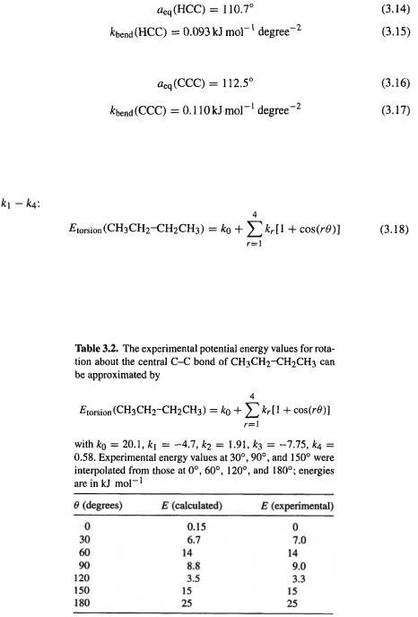
Parameterizing the torsional term. For the ethane case (Fig. 3.4), the equation for energy as a function of dihedral angle can be deduced fairly simply by adjusting the basic equation to give For butane (Fig. 3.5), using Eq. (3.4) and experimenting with a curve-fitting program shows that a reasonably accurate torsional potential energy function can be created with five parameters, and

The values of the parameters are given in Table 3.2. The calculated curve can be made to match the experimental one as closely as desired by using more terms (Fourier analysis).

Parameterizing the nonbonded interactions term. To parameterize Eq. (3.5) we might perform ab initio calculations in which the separation of two atoms or groups in different

Molecular Mechanics 53

molecules (to avoid the complication of concomitant changes in bond lengths and angles) is varied, and fit Eq. (3.5) to the energy vs. distance results. For nonpolar groups this would require quite high-level calculations (chapter 5), as van der Waals or dispersion forces are involved. We shall approximate the nonbonded interactions of methyl groups by the interactions of methane molecules, using experimental values of and , derived from studies of the viscosity or the compressibility of methane. The two methods give slightly different values [7b], but we can use the values

and

Summary of the parameterization of the forcefield terms. The four terms of Eq. (3.1) were parameterized to give:

The parameters k of Eq. (3.25) are given in Table 3.2.

Note that this parameterization is only illustrative of the principles involved; any really viable forcefield would actually be much more sophisticated. The kind we have developed here might at the very best give crude estimates of the energies of alkanes. An accurate, practical forcefield would be parameterized as a best fit to many experimental and/or calculational results, and would have different parameters for different kinds of bonds, e.g. C–C for acyclic alkanes, for cyclobutane and for cyclopropane. A forcefield able to handle not only hydrocarbons would obviously need parameters involving elements other than hydrogen and carbon. Practical forcefields also have different parameters for various atom types, like carbon vs. carbon, or amine nitrogen vs. amide nitrogen. In other words, a different value would be used for, say, stretching involving an C–C bond than for an C–C bond. This is clearly necessary since the force constant of a bond depends on the hybridization of the atoms involved; the IR stretch frequency for the bond comes at roughly while that for the bond is about [8]. Since the vibrational frequency of a bond is proportional to the square root of the force constant, the force constants are in the ratio of about for corresponding atoms, force