

20 Computational Chemistry
the same as they are in the all-staggered conformation. If at every point on the dihedral/ dihedral grid all the other parameters (bond lengths and angles) had been optimized (adjusted to give the lowest possible energy, for that particular calculational method; section 2.4), the result would have been a relaxed PES. In Fig. 2.9 this was not done, but because bond lengths and angles change only slightly with changes in dihedral angles the PES would not be altered much, while the time required for the calculation (for the PES scan) would have been much greater. Figure 2.9 is a nonrelaxed or rigid PES, albeit not very different, in this case, from a relaxed one.
Chemistry is essentially the study of the stationary points on a PES: in studying more or less stable molecules we focus on minima, and in investigating chemical reactions we study the passage of a molecule from a minimum through a transition state to another minimum. There are four known forces in nature: the gravitational force, the strong and the weak nuclear forces, and the electromagnetic force. Celestial mechanics studies the motion of stars and planets under the influence of the gravitational force and nuclear physics studies the behavior of subatomic particles subject to the nuclear forces. Chemistry is concerned with aggregates of nuclei and electrons (with molecules) held together by the electromagnetic force, and with the shuffling of nuclei, followed by their obedient retinue of electrons, around a PES under the influence of this force (with chemical reactions).
The concept of the chemical PES apparently originated with R. Marcelin [6]: in a dissertation-long paper (111 pages) he laid the groundwork for transition-state theory 20 years before the much better-known work of Eyring [5,7]. The importance of Marcelin’s work is acknowledged by Rudolph Marcus in his Nobel Prize (1992) speech, where he refers to “…Marcelin’s classic 1915 theory which came within one small step of the transition state theory of 1935.” The paper was published the year after the death of the author, who seems to have died in World War I, as indicated by the footnote “Tué à l’ennemi en sept 1914”. The first PES was calculated in 1931 by Eyring and Polanyi,2 using a mixture of experiment and theory [8].
2.3 THE BORN–OPPENHEIMER APPROXIMATION
A PES is a plot of the energy of a collection of nuclei and electrons against the geometric coordinates of the nuclei–essentially a plot of molecular energy vs. molecular geometry (or it may be regarded as the mathematical equation that gives the energy as a function of the nuclear coordinates). The nature (minimum, saddle point or neither) of each point was discussed in terms of the response of the energy (first and second derivatives) to changes in nuclear coordinates. But if a molecule is a collection of nuclei and electrons why plot energy vs. nuclear coordinates – why not against electron coordinates? In other words, why are nuclear coordinates the parameters that define molecular geometry? The answer to this question lies in the Born–Oppenheimer approximation.
2Michael Polanyi, Hungarian–British chemist, economist, and philosopher. Born Budapest, 1891. Doctor of medicine 1913, Ph.D. University of Budapest, 1917. Researcher Kaiser-Wilhelm Institute, Berlin, 1920– 1933. Professor of chemistry, Manchester, 1933–1948; of social studies, Manchester, 1948–1958. Professor Oxford, 1958–1976. Best known for book “Personal Knowledge,” 1958. Died Northampton, England, 1976.
The Concept of the Potential Energy Surface 21
Born3 and Oppenheimer4 showed in 1927 [9] that to a very good approximation the nuclei in a molecule are stationary with respect to the electrons. This is a qualitative expression of the principle; mathematically, the approximation states that the Schrödinger equation (chapter 4) for a molecule may be separated into an electronic and a nuclear equation. One consequence of this is that all (!) we have to do to calculate the energy of a molecule is to solve the electronic Schrödinger equation and then add the electronic energy to the internuclear repulsion (this latter quantity is trivial to calculate) to get the total internal energy (see section 4.4.1). A deeper consequence of the Born–Oppenheimer approximation is that a molecule has a shape.
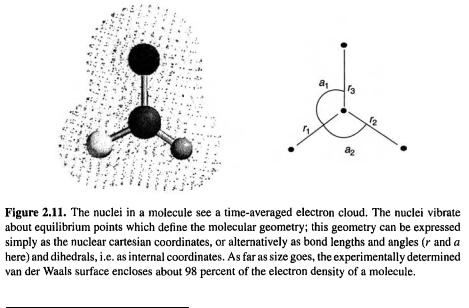
The nuclei see the electrons as a smeared-out cloud of negative charge which binds them in fixed relative positions (because of the mutual attraction between electrons and nuclei in the internuclear region) and which defines the (somewhat fuzzy) surface [10] of the molecule (see Fig. 2.11). Because of the rapid motion of the electrons compared to the nuclei the “permanent” geometric parameters of the molecule are the nuclear coordinates. The energy (and the other properties) of a molecule is a function of the electron coordinates  (x, y, z of each electron); section 5.2), but depends only parametrically on the nuclear coordinates, i.e. for each geometry 1 , 2 , . . . there is a particular energy:
  (x, y, z,...),
 which is a function of x but depends only parametrically on n. Actually, the nuclei are not
3Max Born, German–British physicist. Born in Breslau (now Wroclaw, Poland), 1882, died in Göttingen, 1970. Professor Berlin, Cambridge, Edinburgh. Nobel prize, 1954. One of the founders of quantum mechanics, originator of the probability interpretation of the (square of the) wavefunction (chapter 4).
4J. Robert Oppenheimer, American physicist. Born in New York, 1904, died in Princeton, 1967. Professor California Institute of Technology. Fermi award for nuclear research, 1963. Important contributions to nuclear physics. Director of the Manhattan Project 1943–1945. Victimized as a security risk by senator Joseph McCarthy’s Un-American Activities Committee in 1954. Central figure of the eponymous PBS TV series (Oppenheimer: Sam Waterston).
22 Computational Chemistry
stationary, but execute vibrations of small amplitude about equilibrium positions; it is these equilibrium positions that we mean by the “fixed” nuclear positions. It is only because it is meaningful to speak of (almost) fixed nuclear coordinates that the concepts of molecular geometry or shape [11] and of the PES are valid. The nuclei are much more sluggish than the electrons because they are much more massive (a hydrogen nucleus is about 2000 times more massive than an electron).
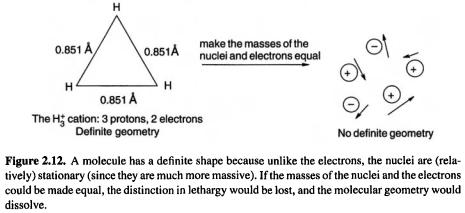
Consider the molecule  made up of three protons and two electrons. Ab initio calculations assign it the geometry shown in Fig. 2.12. The equilibrium positions of the nuclei (the protons) lie at the corners of an equilateral triangle and
  has a definite shape. But suppose the protons were replaced by positrons, which have the same mass as electrons. The distinction between nuclei and electrons, which in molecules rests on mass and not on some kind of charge chauvinism, would vanish. We would have a quivering cloud of flitting particles to which a shape could not be assigned on a macroscopic time scale.
A calculated PES, which we might call a Born–Oppenheimer surface, is normally the set of points representing the geometries, and the corresponding energies, of a collection of atomic nuclei; the electrons are taken into account in the calculations as needed to assign charge and multiplicity (multiplicity is connected with the number of unpaired electrons). Each point corresponds to a set of stationary nuclei, and in this sense the surface is somewhat unrealistic (see section 2.5).
2.4GEOMETRY OPTIMIZATION
The characterization (the “location” or “locating”) of a stationary point on a PES, i.e. demonstrating that the point in question exists and calculating its geometry and energy, is a geometry optimization. The stationary point of interest might be a minimum, a transition state, or, occasionally, a higher-order saddle point. Locating a minimum is often called an energy minimization or simply a minimization, and locating a transition state is often referred to specifically as a transition state optimization. Geometry optimizations are done by starting with an input structure that is believed to resemble (the closer the better) the desired stationary point and submitting this plausible structure to a computer
The Concept of the Potential Energy Surface 23
algorithm that systematically changes the geometry until it has found a stationary point. The curvature of the PES at the stationary point, i.e. the second derivatives of energy with respect to the geometric parameters (section 2.2) may then be determined (section 2.5) to characterize the structure as a minimum or as some kind of saddle point.
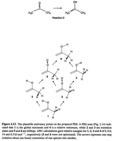
Let us consider a problem that arose in connection with an experimental study. Propanone (acetone) was subjected to ionization followed by neutralization of the radical cation, and the products were frozen in an inert matrix and studied by IR spectroscopy [12]. The spectrum of the mixture suggested the presence of the enol isomer of propanone, 1-propen-2-ol:
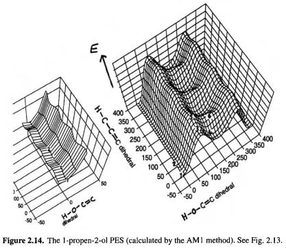
To confirm (or refute) this the IR spectrum of the enol might be calculated (see section 2.5 and the discussions of the calculation of IR spectra in subsequent chapters). But which conformer should one choose for the calculation? Rotation about the C–O and C–C bonds creates six plausible stationary points (Fig. 2.13), and a PES scan (Fig. 2.14)
24 Computational Chemistry
indicated that there are indeed six such species. Examination of this PES shows that the global minimum is structure 1 and that there is a relative minimum corresponding to structure 4. Geometry optimization starting from an input structure resembling 1 gave a minimum corresponding to 1, while optimization starting from a structure resembling 4 gave another, higher-energy minimum, resembling 4. Transition-state optimizations starting from appropriate structures yielded the transition states 2 and 3. These stationary points were all characterized as minima or transition states by second-derivative calculations (section 2.5) (the species 5 and 6 were not located). The calculated IR spectrum of 1 (using the ab initio  method – chapter 5) was in excellent agreement with the observed spectrum of the putative propenol.
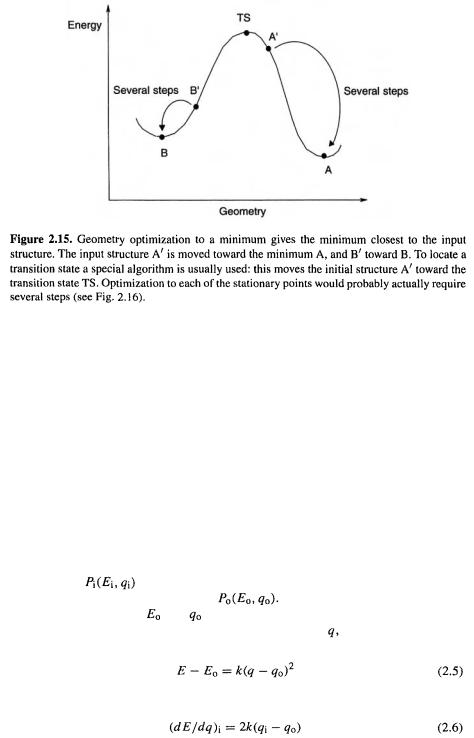
This illustrates a general principle: the optimized structure one obtains is that closest in geometry on the PES to the input structure (Fig. 2.15). To be sure we have found a global minimum we must (except for very simple or very rigid molecules) search a PES (there are algorithms that will do this and locate the various minima). Of course we may not be interested in the global minimum; e.g. if we wish to study the cyclic isomer of ozone (section 2.2) we will use as input an equilateral triangle structure, probably with bond lengths about those of an O–O single bond.
In the propenol example, the PES scan suggested that to obtain the global minimum we should start with an input structure resembling 1, but the exact values of the various bond lengths and angles were unknown (the exact values of even the dihedrals was not known with certainty, although general chemical knowledge made  seem plausible). The actual creation of input structures is
The Concept of the Potential Energy Surface |
25 |
usually done nowadays with an interactive mouse-driven program, in much the same spirit that one constructs plastic models or draws structures on paper. An older alternative is to specify the geometry by defining the various bond lengths, angles and dihedrals, i.e. by using a so-called Z-matrix (internal coordinates).
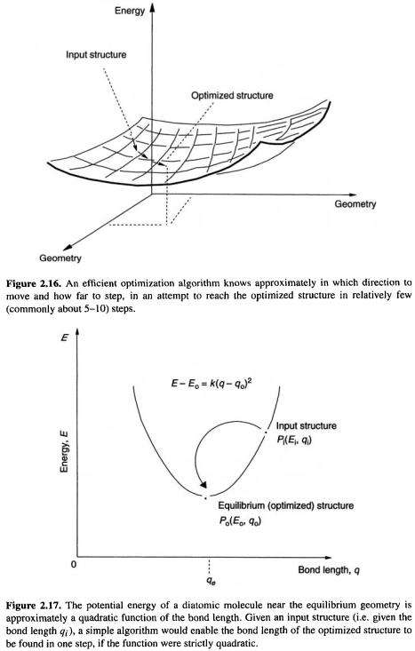
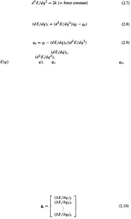
To move along the PES from the input structure to the nearest minimum is obviously trivial on the 1D PES of a diatomic molecule: one simply changes the bond length till that corresponding to the lowest energy is found. On any other surface, efficient geometry optimization requires a sophisticated algorithm. One would like to know in which direction to move, and how far in that direction (Fig. 2.16). It is not possible, in general, to go from the input structure to the proximate minimum in just one step, but modern geometry optimization algorithms commonly reach the minimum in about 10 steps, given a reasonable input geometry. The most widely-used algorithms for geometry optimization [13] use the first and second derivatives of the energy with respect to the geometric parameters. To get a feel for how this works, consider the simple case of a 1D PES, as for a diatomic molecule (Fig. 2.17). The input structure
is at the point |
and the proximate minimum, corresponding to the optimized |
||||
structure being sought, is at the point |
Before the optimization has been |
||||
carried out the values of |
and |
are of course unknown. If we assume that near |
|||
a minimum the potential energy is a quadratic function of |
which is a fairly good |
||||
approximation, then |
|
|
|
|
|
At the input point
26 Computational Chemistry
The Concept of the Potential Energy Surface 27
At all points |
|
|
|
|
From (2.6) and (2.7), |
|
|
|
|
and |
|
|
|
|
Equation (2.9) shows that if we know |
the slope or gradient of the PES at the |
|||
point of the initial structure, |
|
the curvature of the PES (which for a quadratic |
||
curve |
is independent of |
and |
the initial geometry, we can calculate |
the |
optimized geometry. The second derivative of potential energy with respect to geometric displacement is the force constant for motion along that geometric coordinate; as we will see later, this is an important concept in connection with calculating vibrational spectra.
For multidimensional PES’s, i.e. for almost all real cases, far more sophisticated algorithms are used, and several steps are needed since the curvature is not exactly quadratic. The first step results in a new point on the PES that is (probably) closer to the minimum than was the initial structure. This new point then serves as the initial point for a second step toward the minimum, etc. Nevertheless, most modern geometry optimization methods do depend on calculating the first and second derivatives of the energy at the point on the PES corresponding to the input structure. Since the PES is not strictly quadratic, the second derivatives vary from point to point and are updated as the optimization proceeds.
In the illustration of an optimization algorithm using a diatomic molecule, Eq. (2.9) referred to the calculation of first and second derivatives with respect to bond length, which latter is an internal coordinate (inside the molecule). Optimizations are actually commonly done using Cartesian coordinates x, y, z. Consider the optimization of a triatomic molecule like water or ozone in a Cartesian coordinate system. Each of the three atoms has an x, y and z coordinate, giving 9 geometric parameters, the PES would be a 9-dimensional hypersurface on a 10D graph. We need the first and second derivatives of E with respect to each of the 9
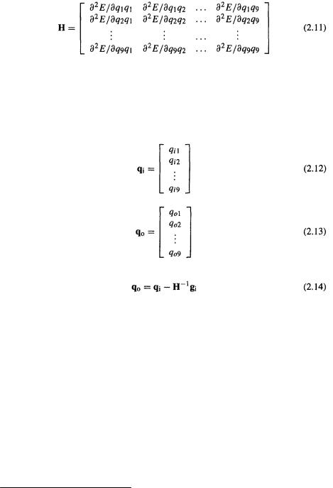
  and these derivatives are manipulated as matrices. Matrices are discussed in section 4.3.3; here we need only know that a matrix is a rectangular array of numbers that can be manipulated mathematically, and that they provide a convenient way of handling sets of linear equations. The first-derivative matrix, the gradient matrix, for the input structure can be written as a column matrix
28 Computational Chemistry
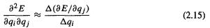
and the second-derivative matrix, the force constant matrix, is
The force constant matrix is called the Hessian.5 The Hessian is particularly important, not only for geometry optimization, but also for the characterization of stationary points as minima, transition states or hilltops, and for the calculation of IR spectra (section 2.5). In the Hessian  as is true for all well-behaved functions, but this systematic notation is preferable: the first subscript refers to the row and the second to the column. The geometry coordinate matrices for the initial and optimized structures are
and
The matrix equation for the general case can be shown to be:
which is somewhat similar to Eq. (2.9) for the optimization of a diatomic molecule. For n atoms we have 3n Cartesians; and
and  are 3n × 1 column matrices and H is a 3n × 3n square matrix; multiplication by the inverse of H rather than division by H is used because matrix division is not defined.
Equation (2.14) shows that for an efficient geometry optimization we need an initial
structure (for  initial gradients (for
  and second derivatives (for H). With an initial “guess” for the geometry (e.g. from a model-building program followed by molecular mechanics) as input, gradients can be readily calculated analytically (from the derivatives of certain integrals). An approximate initial Hessian is often calculated from molecular mechanics (chapter 3). Since the PES is not really exactly quadratic, the first step does not take us all the way to the optimized geometry, corresponding to the matrix
  Rather, we arrive at
  the first calculated geometry; using this geometry a new gradient matrix and a new Hessian are calculated (the gradients are calculated analytically and the second derivatives are updated using the changes in the gradients
– see below). Using  and the new gradient and Hessian matrices a new approximate
5Ludwig Otto Hesse, 1811–1874, German mathematician.
The Concept of the Potential Energy Surface 29
geometry matrix  is calculated. The process is continued until the geometry and/or the gradients (or with some programs possibly the energy) have ceased to change appreciably.
As the optimization proceeds the Hessian is updated by approximating each second derivative as a ratio of finite increments:
i.e. as the change in the gradient divided by the change in geometry, on going from the previous structure to the latest one. Analytic calculation of second derivatives is relatively time-consuming and is not routinely done for each point along the optimization sequence, in contrast to analytic calculation of gradients. A fast lower-level optimization, for a minimum or a transition state, usually provides a good Hessian and geometry for input to a higher-level optimization [14]. Finding a transition state (i.e. optimizing an input structure to a transition state structure) is a more challenging computational problem than finding a minimum, as the characteristics of the PES at the former are more complicated than at a minimum: at the transition state the surface is a maximum in one direction and a minimum in all others, rather than simply a minimum in all directions. Nevertheless, modifications of the minimum-search algorithm enable transitions states to be located, albeit often with less ease than minima.
2.5STATIONARY POINTS AND NORMAL-MODE VIBRATIONS: ZPE
Once a stationary point has been found by geometry optimization, it is usually desirable to check whether it is a minimum, a transition state, or a hilltop. This is done by calculating the vibrational frequencies. Such a calculation involves finding the normal-mode frequencies; these are the simplest vibrations of the molecule, which, in combination, can be considered to result in the actual, complex vibrations that a real molecule undergoes. In a normal-mode vibration all the atoms move in phase with the same frequency: they all reach their maximum and minimum displacements and their equilibrium positions at the same moment. The other vibrations of the molecule are combinations of these simple vibrations. Essentially, a normal-modes calculation is a calculation of the infrared spectrum, although the experimental spectrum is likely to contain extra bands resulting from interactions among normal-mode vibrations.
A nonlinear molecule with n atoms has 3n – 6 normal modes: the motion of each atom can be described by 3 vectors, along the x, y, and z axes of a Cartesian coordinate system; after removing the 3 vectors describing the translational motion of the molecule as a whole (the translation of its center of mass) and the 3 vectors describing the rotation of the molecule (around the 3 principal axes needed to describe rotation for a 3D object of general geometry), we are left with 3n – 6 independent vibrational motions. Arranging these in appropriate combinations gives 3n – 6 normal modes. A linear molecule has 3n – 5 normal modes, since we need subtract only three translational and two rotational vectors, as rotation about the molecular axis does not produce a recognizable
30 Computational Chemistry
change in the nuclear array. So water has 3n – 6 = 3(3) – 6 = 3 normal modes, and HCN has 3n – 5 = 3(3) – 5 = 4 normal modes. For water (Fig. 2.18) mode 1 is a bending mode (the H–O–H angle decreases and increases), mode 2 is a symmetric stretching mode (both O–H bonds stretch and contract simultaneously) and mode 3 is an asymmetric stretching mode (as the bond stretches the
 bond contracts, and vice versa). At any moment an actual molecule of water will be undergoing a complicated stretching/bending motion, but this motion can be considered to be a combination of the three simple normal-mode motions.
Consider a diatomic molecule A–B; the normal-mode frequency (there is only one for a diatomic, of course) is given by [15]:
where |
vibrational “frequency,” actually wavenumber, in |
from deference |
|
to convention we use |
although the cm is not an SI unit, and so the other units |
||
will also be non-SI;  signifies the number of wavelengths that will fit into one cm.
The symbol |
is the Greek letter nu, which resembles an angular vee; could be read |
|||
“nu tilde”; |
“nu bar,” has been used less frequently. |
velocity of light; |
force |
|
constant for the vibration; |
reduced mass of the molecule |
|
||
and |
are the masses of A and B. |
|
|
|
The force |
constant k of a |
vibrational mode is a measure of the “stiffness” |
of the |
|
molecule toward that vibrational mode – the harder it is to stretch or bend the molecule in the manner of that mode, the bigger is that force constant (for a diatomic molecule k simply corresponds to the stiffness of the one bond). The fact that the frequency of a vibrational mode is related to the force constant for the mode suggests that it might be possible to calculate the normal-mode frequencies of a molecule, i.e. the directions and frequencies of the atomic motions, from its force constant matrix (its Hessian). This is indeed possible: matrix diagonalization of the Hessian gives the directional characteristics (which way the atoms are moving), and the force constants themselves, for the vibrations. Matrix diagonalization (section 4.3.3) is a process in which a square matrix A is decomposed into three square matrices, P, D, and  D is a diagonal matrix: as with k in Eq. (2.17) all its off-diagonal elements are zero. P is a premultiplying matrix and
 is the inverse of P. When matrix algebra is applied to physical problems, the diagonal row elements of D are the magnitudes of some physical quantity, and each column of P is a set of coordinates which give a direction associated with that physical quantity. These ideas are made more concrete in the discussion
The Concept of the Potential Energy Surface |
31 |
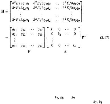
accompanying Eq. (2.17), which shows the diagonalization of the Hessian matrix for a triatomic molecule, e.g. 
Equation (2.17) is of the form  The 9 × 9 Hessian for a triatomic molecule (three Cartesian coordinates for each atom) is decomposed by diagonalization into a P matrix whose columns are “direction vectors” for the vibrations whose force constants are given by the k matrix. Actually, columns 1, 2 and 3 of P and the corresponding
  and
and  of k refer to translational motion of the molecule (motion of the whole molecule from one place to another in space); these three “force constants” are nearly zero. Columns 4, 5 and 6 of P and the corresponding
  and
and  of k refer to rotational motion about the three principal axes of rotation, and are also nearly zero.
Columns 7, 8 and 9 of P and the corresponding |
and |
of k are the direction |
|
vectors and force constants, respectively, for the normal-mode vibrations: |
and |
||
 refer to vibrational modes 1, 2 and 3, while the 7th, 8th, and 9th columns of P are composed of the x, y and z components of vectors for motion of the three atoms in mode 1 (column 7), mode 2 (column 8), and mode 3 (column 9). “Mass-weighting” the force constants, i.e. taking into account the effect of the masses of the atoms (cf. Eq. (2.16) for the simple case of a diatomic molecule), gives the vibrational frequencies. The P matrix is the eigenvector matrix and the k matrix is the eigenvalue matrix from diagonalization of the Hessian H. “Eigen” is a German prefix meaning “appropriate, suitable, actual” and is used in this context to denote mathematically appropriate entities for the solution of a matrix equation. Thus the directions of the normal-mode frequencies are the eigenvectors, and their magnitudes are the mass-weighted eigenvalues, of the Hessian.
Vibrational frequencies are calculated to obtain IR spectra, to characterize stationary points, and to obtain zero point energies (below). The calculation of meaningful frequencies is valid only at a stationary point and only using the same method that was used to optimize to that stationary point (e.g. an ab initio method with a particular correlation level and basis set – see chapter 5). This is because (1) the use of second derivatives as force constants presupposes that the PES is quadratically curved along each geometric coordinate  (Fig. 2.2) but it is only near a stationary point that this is true, and (2) use of a method other than that used to obtain the stationary point presupposes that the PES’s of the two methods are parallel (that they have the same
32 Computational Chemistry
curvature) at the stationary point. Of course, “provisional” force constants at nonstationary points are used in the optimization process, as the Hessian is updated from step to step. Calculated IR frequencies are usually somewhat too high, but (at least for ab initio and density functional calculations) can be brought into reasonable agreement with experiment by multiplying them by an empirically determined factor, commonly about 0.9 [16] (see the discussion of frequencies in chapters 5–7).
A minimum on the PES has all the normal-mode force constants (all the eigenvalues of the Hessian) positive: for each vibrational mode there is a restoring force, like that of a spring. As the atoms execute the motion, the force pulls and slows them till they move in the opposite direction; each vibration is periodic, over and over. The species corresponding to the minimum sits in a well and vibrates forever (or until it acquires enough energy to react). For a transition state, however, one of the vibrations, that along the reaction coordinate, is different: motion of the atoms corresponding to this mode takes the transition state toward the product or toward the reactant, without a restoring force. This one “vibration” is not a periodic motion but rather takes the species through the transition state geometry on a one-way journey. Now, the force constant is the first derivative of the gradient or slope (the derivative of the first derivative); examination of Fig. 2.8 shows that along the reaction coordinate the surface slopes downward, so the force constant for this mode is negative. A transition state (a first-order saddle point) has one and only one negative normal-mode force constant (one negative eigenvalue of the Hessian). Since a frequency calculation involves taking the square root of a force constant (Eq. (2.16)), and the square root of a negative number is an imaginary number, a transition state has one imaginary frequency, corresponding to the reaction coordinate. In general an nth-order saddle point (an nth-order hilltop) has n negative normal-mode force constants and so n imaginary frequencies, corresponding to motion from one stationary point of some kind to another.
A stationary point could of course be characterized just from the number of negative force constants, but the mass-weighting requires much less time than calculating the force constants, and the frequencies themselves are often wanted anyway, e.g. for comparison with experiment. In practice one usually checks the nature of a stationary point by calculating the frequencies and seeing how many imaginary frequencies are present; a minimum has none, a transition state one, and a hilltop more than one. If one is seeking a particular transition state the criteria to be satisfied are:
1.It should look right. The structure of a transition state should lie somewhere between that of the reactants and the products; e.g. the transition state for the unimolecular isomerization of HCN to HNC shows an H bonded to both C and N by an unusually long bond, and the CN bond length is in-between that of HCN and HNC.
2.It must have one and only one imaginary frequency (some programs indicate this as a negative frequency, e.g.–  instead of the correct
3.The imaginary frequency must correspond to the reaction coordinate. This is usually clear from animation of the frequency (the motion, stretching, bending, twisting, corresponding to a frequency may be visualized with a variety of programs). For example, the transition state for the unimolecular isomerization of HCN to HNC shows an imaginary frequency which when animated clearly shows the H migrating between the C and the N. Should it not be clear from animation which two species the