


Semiempirical Calculations 369
potentials, whether visualized as regions of space or mapped onto van der Waals surfaces, are usually qualitatively the same for AM1 and PM3 as for ab initio methods. Atoms-in-molecules calculations are not viable for SE methods, because the core orbitals, lacking in these methods, are important for AIM calculations.
Dipole moments
Hehre’s extensive survey of practical computational methods reports the results of ab initio and DFT single point dipole moment  calculations on AM1 geometries [74]. There does not appear to be much advantage to calculating HF/6-31G* dipole moments on HF/6-31G* geometries (HF/6-31G*//HF/6-31G* calculations) rather than on the much more quicklyobtained AM1 geometries (HF/6-31G*//AM1 calculations). Indeed, even the relatively time-consuming MP2/6-31G*//MP2/6-31G* calculations seem to offer little advantage over fast HF/6-31G*//AM1 calculations as far as dipole moments are concerned (Tables 2.19 and 2.21 in Ref. [74]). This is consistent with our finding that AM1 geometries are quite good (section 6.3.1). Table 6.5 compares calculated and experimental dipole moments for 10 molecules,
370 Computational Chemistry
using these methods: AM1 (using the AM1 method to calculate  for the AM1 geometry, AM1//AM1), HF/6-31*//AM1, PM3 (PM3//PM3), HF/6-31G*//PM3, and MP2/6-31G* (MP2/6-31G*//MP2/6-31G*). For this set of molecules, the smallest deviation from experiment, as judged by the arithmetic mean of the absolute deviations from the experimental values, is shown by the AM1 calculation (0.21 Debyes), and the largest deviation is shown by the “highest” method, MP2/6-31G* (0.34 D). The other three methods give essentially the same errors (0.27–0.29 D). It is of course possible that AM1 gives the best results (for this set on molecules, at least) because errors in geometry and errors in the calculation of the electron distribution cancel. A study of 196 C, H, N, O, F, Cl, Br, I molecules gave these mean absolute errors: AM1, 0.35 D; PM3, 0.40D; SAM1, 0.32 D [50]. Another study with 125 H, C, N, O, F, A1, Si, P, S, Cl, Br, I molecules gave mean absolute errors of: AM1, 0.35 D and PM3, 0.38D [44]. So with these larger samples the AM1 errors were somewhat bigger. Nevertheless, all these results taken together do indicate that unless one is prepared to use the slower approach of large basis sets with density functional (chapter 7) methods (errors of ca. 0.1 D [75]; this paper also gives some results for ab initio calculations), AM1 dipole moments using AM1 geometries may be as good a way as any to calculate this quantity.

Semiempirical Calculations 371
This applies, of course, only to conventional molecules; molecules of exotic structure (note the remarks for the geometries of hypervalent molecules and molecules ofunusual structure in section 6.3.1) may defy accurate SE predictions.
Charges and bond orders
The conceptual and mathematical bases of these concepts were outlined in chapter 5 (section 5.5 4). We saw that unlike, say, frequencies and dipole moments, charges and bond orders cannot even in principle be measured experimentally; as physicists say, they are not observables. Thus there are no “right” values to calculate, and in fact no single, correct, definitions of these terms, since as with ab initio calculations, SE charges and bond orders can be defined in various ways. The concepts are nevertheless useful, and electrostatic potential charges and Löwdin bond orders are preferred nowadays to the Mulliken parameters.
Figure 6.9 shows charges and bond orders calculated for an enolate (the conjugate base of ethenol or vinyl alcohol) and for a protonated enone system (protonated propenal). Consider first Mulliken charges and bond orders of the enolate (Fig. 6.9A). The AM1 and PM3 charges, which are essentially the same, are a bit surprising in that the carbon which shares charge with the oxygen in the alternative resonance structure is given a bigger charge than the oxygen; intuitively, one expects most of the negative charge to be on the more electronegative atom, oxygen (this “defect” of AM1 and PM3 has been noted by Anh et al. [76]). The HF/3-21G method gives the oxygen the bigger charge (–0.80 vs. –0.67). The two SE and the HF methods all give C/C and C/O bond orders of about 1.5; this, and the rough equality of O and C charges, suggests approximately equal contributions from the O-anion and C-anion resonance structures.
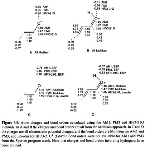
372 Computational Chemistry
The Mulliken charges of the protonated enone system (Fig. 6.9B) make the oxygen negative, which may seem surprising. However, this is normal for protonated oxygen and nitrogen (though not protonated sulfur and phosphorus): the hetero atom in  and in
  is calculated to be negative (i.e. the positive charge is on the hydrogens) and the hetero atom is also negative in
  and
and  On the oxygen and the carbon furthest from the oxygen
  the HF/3-21G charges differ considerably from the SE ones: the HF calculations make the O much more negative, and make
  negative, suggesting that they place more positive charge on the hydrogens than do the semiempirical calculations (in all cases the charge on
  is 0.3–0.5). The three methods do not differ as greatly in their bond order results, although HF method makes the formal C/O double bond essentially a single bond (bond order 1.18).
Finally, electrostatic potential (ESP) charges and, for the HF/3-21G calculations, Löwdin bond orders, are shown (Figs 6.9C and D). For the enolate, all three methods make the ESP charge on carbon more negative than that on oxygen, but the bond orders