


The Concept of the Potential Energy Surface 13
The slice could be made holding one or the other of the two geometric parameters constant, or it could involve both of them, giving a diagram in which the geometry axis is a composite of more than one geometric parameter. Analogously, we can take a 3D slice of the hypersurface for HOF (Fig. 2.6) or even a more complex molecule and use an E vs.  diagram to represent the PES; we could even use a simple 2D diagram, with q representing one, two or all of the geometric parameters. We shall see that these 2D and particularly 3D graphs preserve qualitative and even quantitative features of the mathematically rigorous but unvisualizable
 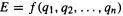 n-dimensional hypersurface.
2.2STATIONARY POINTS
Potential energy surfaces are important because they aid us in visualizing and understanding the relationship between potential energy and molecular geometry, and in understanding how computational chemistry programs locate and characterize structures of interest. Among the main tasks of computational chemistry are to determine the structure and energy of molecules and of the transition states involved in chemical

14 Computational Chemistry
reactions: our “structures of interest” are molecules and the transition states linking them. Consider the reaction
A priori, it seems reasonable that ozone might have an isomer (call it isoozone) and that the two could interconvert by a transition state as shown in reaction (1). We can depict this process on a PES. The potential energy E must be plotted against only two geometric parameters, the bond length (we may reasonably assume that the two O–O bonds of ozone are equivalent, and that these bond lengths remain equal throughout the reaction) and the O–O–O bond angle. Figure 2.7 shows the PES for reaction (1), as calculated by the AM 1 semiempirical method (chapter 6; the AM 1 method is unsuitable for quantitative treatment of this problem, but the PES shown makes the point), and shows how a 2D slice from this 3D diagram gives the energy/reaction coordinate type of diagram commonly used by chemists. The slice goes along the lowest-energy path connecting ozone, isoozone and the transition state, i.e. along the reaction coordinate,

The Concept of the Potential Energy Surface |
15 |
and the horizontal axis (the reaction coordinate) of the 2D diagram is a composite of O–O bond length and O–O–O angle. In most discussions this horizontal axis is left quantitatively undefined; qualitatively, the reaction coordinate represents the progress of the reaction. The three species of interest, ozone, isoozone, and the transition state linking these two, are called stationary points. A stationary point on a PES is a point at which the surface is flat, i.e. parallel to the horizontal line corresponding to the one geometric parameter (or to the plane corresponding to two geometric parameters, or to the hyperplane corresponding to more than two geometric parameters). A marble placed on a stationary point will remain balanced, i.e. stationary (in principle; for a transition state the balancing would have to be exquisite indeed). At any other point on a potential surface the marble will roll toward a region of lower potential energy.
16 Computational Chemistry
Mathematically, a stationary point is one at which the first derivative of the potential energy with respect to each geometric parameter is zero:
Partial derivatives, |
are written here rather than |
to emphasize that |
each derivative is with respect to just one of the variables |
of which E is a function. |
|
Stationary points that correspond to actual molecules with a finite lifetime (in contrast to transition states, which exist only for an instant), like ozone or isoozone, are minima, or energy minima: each occupies the lowest-energy point in its region of the PES, and any small change in the geometry increases the energy, as indicated in Fig. 2.7. Ozone is a global minimum, since it is the lowest-energy minimum on the whole PES, while isoozone is a relative minimum, a minimum compared only to nearby points on the surface. The lowest-energy pathway linking the two minima, the reaction coordinate or intrinsic reaction coordinate (IRC; dashed line in Fig. 2.7) is the path that would be followed by a molecule in going from one minimum to another should it acquire just enough energy to overcome the activation barrier, pass through the transition state, and reach the other minimum. Not all reacting molecules follow the IRC exactly: a molecule with sufficient energy can stray outside the IRC to some extent [3].
Inspection of Fig. 2.7 shows that the transition state linking the two minima represents a maximum along the direction of the IRC, but along all other directions it is a minimum. This is a characteristic of a saddle-shaped surface, and the transition state is called a saddle point (Fig. 2.8). The saddle point lies at the “center” of the saddle-shaped region and is, like a minimum, a stationary point, since the PES at that point is parallel to the plane defined by the geometry parameter axes: we can see that a marble placed (precisely) there will balance. Mathematically, minima and saddle points differ in that although both are stationary points (they have zero first derivatives; Eq. (2.1)), a minimum is a minimum in all directions, but a saddle point is a maximum along the

The Concept of the Potential Energy Surface |
17 |
reaction coordinate and a minimum in all other directions (examine Fig. 2.8). Recalling that minima and maxima can be distinguished by their second derivatives, we can write:
For a minimum
for all q.
For a transition state
for all q, except along the reaction coordinate, and
along the reaction coordinate.
The distinction is sometimes made between a transition state and a transition structure [4]. Strictly speaking, a transition state is a thermodynamic concept, the species an ensemble of which are in a kind of equilibrium with the reactants in Eyring’s1 transitionstate theory [5]. Since equilibrium constants are determined by free energy differences, the transition state, within the strict use of the term, is a free energy maximum along the reaction coordinate (in so far as a single species can be considered representative of the ensemble). This species is also often (but not always [5]) also called an activated complex. A transition structure, in strict usage, is the saddle point (Fig. 2.8) on a theoretically calculated (e.g. Fig. 2.7) PES. Normally such a surface is drawn through a set of points each of which represents the enthalpy of a molecular species at a certain geometry; recall that free energy differs from enthalpy by temperature times entropy. The transition structure is thus a saddle point on an enthalpy surface. However, the energy of each of the calculated points does not normally include the vibrational energy, and even at 0 K a molecule has such energy (ZPE: Fig. 2.2, and section 2.5). The usual calculated PES is thus a hypothetical, physically unrealistic surface in that it neglects vibrational energy, but it should qualitatively, and even semiquantitatively, resemble the vibrationally-corrected one since in considering relative enthalpies ZPEs at least roughly cancel. In accurate work ZPEs are calculated for stationary points and added to the “frozen-nuclei” energy of the species at the bottom of the reaction coordinate curve in an attempt to give improved relative energies which represent enthalpy differences at 0 K (and thus, at this temperature where entropy is zero, free energy differences also; Fig. 2.19). It is also possible to calculate enthalpy and entropy differences, and thus free energy differences, at, say, room temperature (section 5.5.2). Many chemists do not routinely distinguish between two terms, and in this book the commoner term, transition state, is used. Unless indicated otherwise, it will mean a calculated geometry, the saddle point on a hypothetical vibrational-energy-free PES.
1 Henry Eyring, American chemist. Born Colonia Juarárez, Mexico, 1901. Ph.D. University of California, Berkeley, 1927. Professor Princeton, University of Utah. Known for his work on the theory of reaction rates and on potential energy surfaces. Died Salt Lake City, Utah, 1981.
18 Computational Chemistry
The geometric parameter corresponding to the reaction coordinate is usually a composite of several parameters (bond lengths, angles and dihedrals), although for some reactions one or two may predominate. In Fig. 2.7, the reaction coordinate is a composite of the O–O bond length and the O–O–O bond angle.
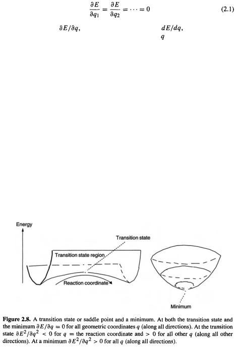
A saddle point, the point on a PES where the second derivative of energy with respect to one and only geometric coordinate (possibly a composite coordinate) is negative, corresponds to a transition state. Some PES’s have points where the second derivative of energy with respect to more than one coordinate is negative; these are higher-order saddle points or hilltops: e.g. a second-order saddle point is a point on the PES which is a maximum along two paths connecting stationary points. The propane PES, Fig. 2.9, provides examples of a minimum, a transition state and a hilltop – a second-order saddle point in this case. Figure 2.10 shows the three stationary points in more detail. The “doubly-eclipsed” conformation (A), in which there is eclipsing as viewed along the C1–C2 and the C3–C2 bonds (the dihedral angles are 0° viewed along these bonds) is a second-order saddle point because single bonds do nor like to eclipse single bonds and rotation about the C1–C2 and the C3–C2 bonds will remove this eclipsing: there are two possible directions along the PES which lead, without a barrier, to lower-energy regions, i.e. changing the H–C1/C2–C3 dihedral and changing the H–C3/C2–C1 dihedral. Changing one of these leads to a “singly-eclipsed” conformation (B) with only one offending eclipsing CH3–CH2 arrangement, and this

The Concept of the Potential Energy Surface |
19 |
is a first-order saddle point, since there is now only one direction along the PES which leads to relief of the eclipsing interactions (rotation around C3–C2). This route gives a conformation C which has no eclipsing interactions and is therefore a minimum. There are no lower-energy structures on the  PES and so C is the global minimum.
The geometry of propane depends on more than just two dihedral angles, of course; there are several bond lengths and bond angles and the potential energy will vary with changes in all of them. Figure 2.9 was calculated by varying only the dihedral angles associated with the C1–C2 and C2–C3 bonds, keeping the other geometrical parameters