


122 Computational Chemistry
Diagonalization of the four-basis-function matrix of Eq. (4.65) gives
The energy levels and MOs from these results are shown in Fig. 4.17. Note that all these matrix diagonalizations yield orthonormal eigenvectors:  and
and as required the fact that the Fock matrices are symmetric (see the discussion of matrix diagonalization in section 4.3.3).
4.3.5 The simple Hückel method – applications
Applications of the SHM are discussed in great detail in several books [21]; here we will deal only with those applications which are needed to appreciate the utility of the method and to smooth the way for the discussion of certain topics (like bond orders and atomic charges) in later chapters. We will discuss: the nodal properties of the MOs; stability as indicated by energy levels and aromaticity (the 4n + 2 rule); resonance energies; and bond orders and atomic charges.
The nodal properties of the MOs
A node of an MO is a plane at which, as we proceed along the sequence of basis functions, the sign of the wavefunction changes (Figs 4.15–4.17). For a given molecule,
the number of nodes in the |
orbitals increases with the energy. In the two-orbital |
||||||
system (Fig. 4.15), |
has zero nodes and |
has one node. In the three-orbital system |
|||||
(Fig. 4.16), |
and |
have zero, one and two nodes, respectively. In the cyclic |
|||||
four-orbital system (Fig. 4.17), |
has zero nodes, |
and |
which are degenerate |
||||
(of the same energy) each have one node (one nodal plane), and |
has two nodes. |
||||||
In a given molecule, the energy of the MOs increases with the number of nodes. The nodal properties of the SHM  orbitals form the basis of one of the simplest ways of

Introduction to Quantum Mechanics 123
understanding the predictions of the Woodward–Hoffmann orbital symmetry rules [38]. For example, the thermal conrotatary and disrotatary ring closure/opening of polyenes can be rationalized very simply in terms of the symmetry of the highest occupied  MO of the open-chain species. That the highest
  MO should dominate the course of this kind of reaction is indicated by more detailed considerations (including extended Hückel calculations) [38]. Figure 4.18 shows the situation for the ring closure of a 1,3-butadiene to a cyclobutene. The phase (+ or –) of the
  HOMO
HOMO  at the end carbons (the atoms that bond) is opposite on each face, because this orbital has one node in the middle of the
 chain. You can see this by sketching the MO as the four AOs contributing to it, or even – remembering the node – drawing just the end AOs. For the electrons in
  to bond, the end groups must rotate in the same sense (conrotation) to bring orbital lobes of the same phase together. Remember that plus and minus phase has nothing to do with electric charge, but is a consequence of the wave nature of electrons (section 4.2.6): two electron waves can reinforce one another and form a bonding pair if they are “vibrating in phase”; an out-of-phase interaction represents an antibonding situation. Rotation in opposite senses (disrotation) would bring opposite-phase lobes together, an antibonding situation. The mechanism of the reverse reaction is simply the forward mechanism in reverse, so the fact that the thermodynamically favored process is the ring-opening of a cyclobutene simply means that the cyclobutene shown would open to the butadiene shown on heating. Photochemical processes can also be

124 Computational Chemistry
accommodated by the Woodward–Hoffmann orbital symmetry rules if we realize that absorption of a photon creates an electronically excited molecule in which the previous lowest unoccupied MO (LUMO) is now the HOMO. For more about orbital symmetry and chemical reactions see, e.g. the book by Woodward and Hoffmann [38].
Stability as indicated by energy levels and aromaticity
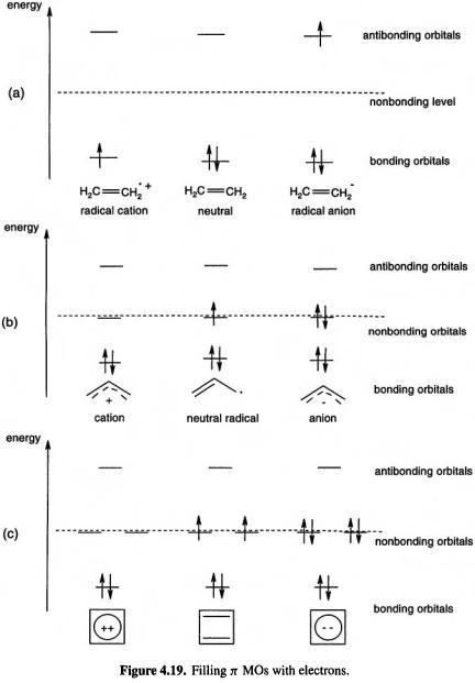
The MO energy levels obtained from an SHM calculation must be filled with electrons according to the species under consideration. For example, the neutral ethene molecule has two electrons, so the diagrams of Fig. 4.19(a) (cf. Fig. 4.15) with one, two and three
  electrons, would refer to the cation, the neutral and the anion. We might expect the neutral, with its bonding
  orbital
  full and its antibonding
  orbital
  empty, to be resistant to oxidation (which would require removing electronic charge from the low-energy
  and to reduction (which would require adding electronic charge to the
high-energy 
The propenyl (allyl) system has two, three or four electrons, depending on whether we are considering the cation, radical or anion (Fig. 4.19(b); cf. Fig. 4.16). The cation
Introduction to Quantum Mechanics 125
might be expected to be resistant to oxidation, which requires removing an electron from a low-lying  orbital
  and to be moderately readily reduced, as this involves adding an electron to the nonbonding
 orbital
  a process that should not be strongly favorable or unfavorable. The radical should be easier to oxidize than the cation, for this

126 Computational Chemistry
requires removing an electron from a nonbonding, rather than a lower-lying bonding, orbital, and the ease of reduction of the radical should be roughly comparable to that of the cation, as both can accommodate an electron in a nonbonding orbital. The anion should be oxidized with an ease comparable to that of the radical (removal of an
electron from the nonbonding |
but be harder to reduce (addition of an electron to |
the antibonding |
|
The cyclobutadiene system |
(Fig. 4.19(c); cf. Fig. 4.17) can be envisaged with, |
amongst others, two (the dication), four (the neutral molecule) and six  (the dianion) electrons. The predictions one might make for the behavior of these three species toward redox reactions are comparable to those just outlined for the propenyl cation, radical and anion, respectively (note the analogous occupancy of bonding, nonbonding and antibonding orbitals). The neutral cyclobutadiene molecule is, however, predicted by the SHM to have an unusual electronic arrangement for a diene:
in filling the |
orbitals, from the lowest-energy one up, one puts electrons of the |
||
same spin into the degenerate |
and |
in accordance with Hund’s rule of max- |
|
imum multiplicity. Thus the SHM predicts that cyclobutadiene will be a diradical, with two unpaired electrons of like spin. Actually, more advanced calculations [39] indicate, and experiment confirms, that cyclobutadiene is a singlet molecule with two single and two double C/C bonds. A square cyclobutadiene diradical with four 1.5 C/C bonds would distort to a rectangular, closed-shell (i.e. no unpaired electrons) molecule with two single and two double bonds (Fig. 4.20). This could have been predicted by augmenting the SHM result with a knowledge of the phenomenon known as the Jahn–Teller effect [40]: cyclic systems (and certain others) with an odd number of electrons in degenerate (equal-energy) MOs will distort to remove the degeneracy.
Introduction to Quantum Mechanics 127
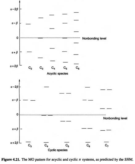
What general pattern of MOs emerges from the SHM? Acyclic  systems (ethene, the propenyl system, 1,3-butadiene, etc.), have MOs distributed singly and evenly on each side of the nonbonding level; the odd-AO systems also have one nonbonding MO (Fig. 4.21). Cyclic
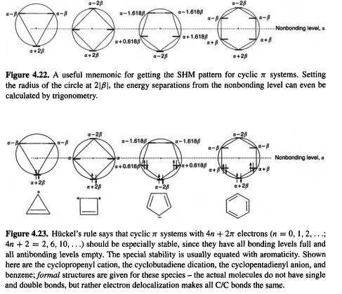
  systems (the cyclopropenyl system, cyclobutadiene, the cyclopentadienyl system, benzene, etc.) have a lowest MO and pairs of degenerate MOs, ending with one highest or a pair of highest MOs, depending on whether the number of MOs is even or odd. The total number of MOs is always equal to the number of basis functions, which in the SHM is, for organic polyenes, the number of p orbitals (Fig. 4.21). The pattern for cyclic systems can be predicted qualitatively simply by sketching the polygon, with one vertex down, inside a circle (Fig. 4.22). If the circle is of radius
  the energies can even be calculated by trigonometry [41 ]. It follows from this
128 Computational Chemistry
pattern that cyclic species (not necessarily neutral) with 2, 6, 10, …  electrons have filled
 MOs and might be expected to show particular stability, analogously to the filled AOs of the unreactive noble gases (Fig. 4.23). The archetype of such molecules is, of course, benzene, and the stability is associated with the general collection of properties called aromaticity [17]. These results, which were first perceived by Hückel [ 19] (1931– 1937), are summarized in a rule called the 4n + 2 rule or Hückel’s rule, although the 4n + 2 formulation was evidently actually due to Doering and Knox (1954) [42]. This says that cyclic arrays of
 -hybridized atoms with
  electrons are characteristic of aromatic molecules; the canonical aromatic molecule benzene with six
 electrons corresponds to n = 1. For neutral molecules with formally fully conjugated perimeters this amounts to saying that those with an odd number of C/C double bonds are aromatic and those with an even number are antiaromatic (see resonance energies, below).
Hückel’s rule has been abundantly verified [17] notwithstanding the fact that the SHM, when applied without regard to considerations like the Jahn–Teller effect (see above) incorrectly predicts 4n species like cyclobutadiene to be triplet diradicals. The Hückel rule also applies to ions; for example, the cyclopropenyl with system two  electrons, the cyclopropenyl cation, corresponds to n = 0, and is strongly aromatic.

Introduction to Quantum Mechanics 129
Other aromatic species are the cyclopentadienyl anion (six  electrons,
  Hückel predicted the enhanced acidity of cyclopentadiene) and the cycloheptatrienyl cation. Only reasonably planar species can be expected to provide the AO overlap need for cyclic electron delocalization and aromaticity, and care is needed in applying the rule.
Resonance energies
The SHM permits the calculation of a kind of stabilizing energy, or, more accurately, an energy that reflects the stability of molecules. This energy is calculated by comparing the total electronic energy of the molecule in question with that of a reference compound, as shown below for the propenyl systems, cyclobutadiene, and the cyclobutadiene dication.
The propenyl cation, Fig. 4.19(b); cf. Fig. 4.16. If we take the total  electronic energy of a molecule to be simply the number of electrons in a
  MO times the energy level of the orbital, summed over occupied orbitals (a gross approximation, as it ignores interelectronic repulsion), then for the propenyl cation
We want to compare this energy with that of two electrons in a normal molecule with no special features (the propenyl cation has the special feature of an empty p orbital adjacent to the formal C/C double bond), and we choose neutral ethene for our reference energy (Fig. 4.15)
The stabilization energy is then
Since  is negative, the
  electronic energy of the propenyl cation is calculated to be below that of ethene: providing an extra, empty p orbital for the electron pair causes the energy to drop. Actually, resonance energy is usually presented as a positive quantity, e.g.
  We can interpret this as
  below a reference system. To avoid a negative quantity in SHM calculations like these, we can use
  instead of
The propenyl radical, Fig. 4.16. The total  electronic energy by the SHM is
For the reference energy we use one ethene molecule and one nonbonding p electron (like the electron in a methyl radical):
The stabilization energy is then
130 Computational Chemistry
The propenyl anion. An analogous calculation (cf. Fig. 4.16, with four electrons for the anion) gives
Thus the SHM predicts that all three propenyl species will be lower in energy than if the  electrons were localized in the formal double bond and (for the radical and anion) in one p orbital. Because this lower energy is associated with the ability of the electrons to spread or be delocalized over the whole
  system, what we have called E(stab) is often denoted as the delocalization energy, and designated
  Note that
  (or
(or  is always some multiple of
  (or is zero). Since electron delocalization can be indicated by the familiar resonance symbolism the Hückel delocalization energy is often equated with resonance energy, and designated
  The accord between calculated delocalization and the ability to draw resonance structures is not perfect, as indicated by the next example.
Cyclobutadiene (Fig. 4.17). The total  electronic energy is
Using two ethene molecules as our reference system:
and so for E(stab)  we get
Cyclobutadiene is predicted by this calculation to have no resonance energy, although we can readily draw two “resonance structures” exactly analogous to the Kekulé struc-
tures of benzene. The SHM predicts a resonance energy of |
for benzene. Equating |
||
with the commonly-quoted resonance energy of |
for |
||
benzene gives a value of |
for |
but this should be taken with more than |
|
a grain of salt, for outside a closely related series of molecules, |
has little or no quan- |
||
titative meaning [43]. However, |
in contrast to the failure of simple resonance theory |
||
in predicting aromatic stabilization (and other chemical phenomena) [44], the SHM is quite successful.
The cyclobutadiene dication (cf. Fig. 4.17). The total  electronic energy is
Using one ethene molecule as the reference:
and so
Introduction to Quantum Mechanics 131
Thus the stabilization energy calculation agrees with the deduction from the disposition of filled MOs (i.e. with the 4n + 2 rule) that the cyclobutadiene dication should be stabilized by electron delocalization, which is in some agreement with experiment [45].
More sophisticated calculations indicate that cyclic 4n systems like cyclobutadiene (where planar; cyclooctatetraene, for example, is buckled by steric factors and is simply an ordinary polyene) are actually destabilized by  electronic effects: their resonance energy is not just zero, as predicted by the SHM, but less than zero. Such systems are antiaromatic [17,46].
Bond orders
The meaning of this term is easy to grasp in a qualitative, intuitive way: an ideal single bond has a bond order of one, and ideal double and triple bonds have bond orders of two and three, respectively. Invoking Lewis electron-dot structures, one might say that the order of a bond is the number of electron pairs being shared between the two bonded atoms. Calculated quantum mechanical bond orders should be more widely applicable than those from the Lewis picture, because electron pairs are not localized between atoms in a clean pairwise manner; thus a weak bond, like a hydrogen bond or a long single bond, might be expected to have a bond order of less than one. However, there is no unique definition of bond order in computational chemistry, because there seems to be no single, correct method to assign electrons to particular atoms or pairs of atoms [47]. Various quantum mechanical definitions of bond order can be devised [48], based on basis-set coefficients. Intuitively, these coefficients for a pair of atoms should be relevant to calculating a bond order, since the bigger the contribution two atoms make to the wavefunction (whose square is a measure of the electron density; section 4.2.6), the bigger should be the electron density between them. In the SHM the order of a bond between two atoms  and
and  is defined as
Here the 1 denotes the single bond of the ubiquitous spectator  bond framework, which is taken as always contributing a
  bond order of unity. The other term is the
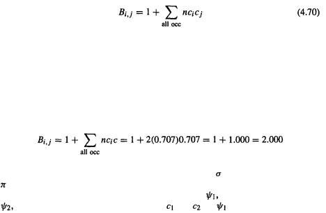
  bond order; its value is obtained by summing over all the occupied MOs the number of electrons n in each of these MOs times the product of the c’s of the two atoms for each MO. This is illustrated in the following examples.
Ethene. The occupied orbital is  which has 2 electrons), and the coefficients of
  and
and  for this orbital are 0.707, 0.707 (Eq. (4.66)). Thus
which is reasonable for a double bond. The order of the |
bond is 1 and that of the |
bond is 1. |
|
The ethene radical anion. The occupied orbitals are |
which has 2 electrons, and |
which has 1 electron; the coefficients of and for |
are 0.707, 0.707 and for |
132 Computational Chemistry
 0.707, –0.707 (Eq. (4.66)). Thus
The  bond order of 0.500 (1,500 –
 bond order) accords with two electrons in the bonding MO and one electron in the antibonding orbital.
Atomic charges
In an intuitive way, the charge on an atom might be thought to be a measure of the extent to which the atom repels or attracts a charged probe near it, and to be measurable from the energy it takes to bring a probe charge from infinity up to near the atom. However, this would tell us the charge at a point outside the atom, for example a point on the van der Waals surface of the molecule, and the repulsive or attractive forces on the probe charge would be due to the molecule as a whole. Although atomic charges are generally considered to be experimentally unmeasurable, chemists find the concept very useful (thus calculated charges are used to parameterize molecular mechanics force fields – chapter 3), and much effort has gone into designing various definitions of atomic charge [47,48]. Intuitively, the charge on an atom should be related to the basis set coefficients of the atom, since the more the atom contributes to a multicenter wavefunction (one with contributions from basis functions on several atoms), the more it might be expected to lose electronic charge by delocalization into the rest of the molecule (cf. the discussion of bond order above). In the SHM the charge on an atom
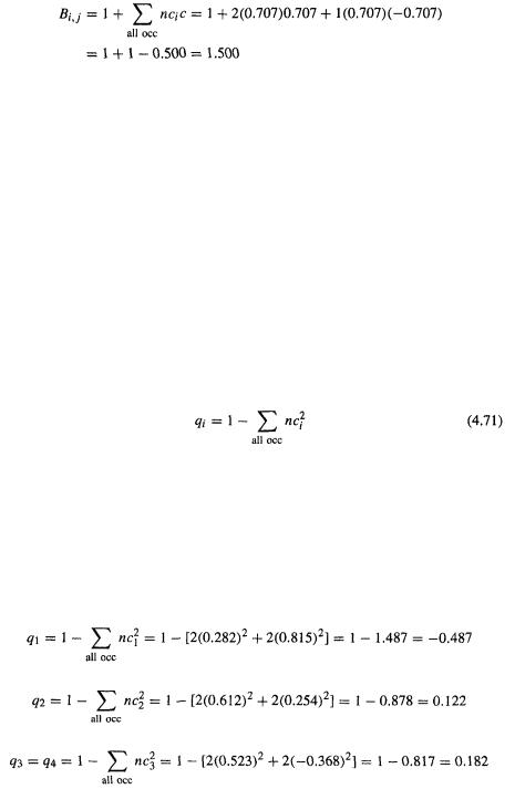
 is defined as (cf. Eq. (4.70))
The summation term is the charge density, and is a measure of the electronic charge on the molecule due to the  electrons. For example, having no
  electrons (an empty p orbital, formally a cationic carbon) would mean a
  electron charge density of zero; subtracting this from unity gives a charge on the atom of +1. Again, having two
 electrons in a p orbital would mean a
 electron charge density of 2 on the atom; subtracting this from unity gives a charge on the atom of – 1 (a filled p orbital, formally an anionic carbon). The application of Eq. (4.71) will be illustrated using methylenecyclopropene (Fig. 4.24).
Methylenecyclopropene (Fig. 4.24).