


Density Functional Calculations 413
high-level ab initio calculations are more trustworthy than DFT, presumably because current DFT functionals are really semiempirical.
7.3.3 Frequencies
The general remarks and theory about frequencies that were given in section 5.5.2.2d apply to DFT frequencies also. As with ab initio frequency calculations, but unlike semiempirical, one reason for calculating DFT frequencies is to get zero-point energies to correct the frozen-nuclei energies. The frequencies are also used to characterize the stationary point as a minimum, transition state, etc., and to predict the IR spectrum. As usual the wavenumbers ("frequencies") are the mass-weighted eigenvalues of the hessian, and the intensities are calculated from changes in dipole moment incurred by the vibrations.
Unlike ab initio and semiempirical frequencies, DFT frequencies are not always significantly lower than observed ones (indeed, calculated values slightly higher than experimental frequencies have been reported). Here are some correction factors that have been calculated for various functionals, as well as for some ab initio and semiempirical methods (slightly different factors were recommended for accurate calculations of ZPE) [62]; except for HF/3-21G the basis set for the ab initio and DFT methods is6-31G*:
HF/3-21G |
HF/6-31G* |
MP2(FC) |
AMI BLYP BP86 B3LYP |
B3PW91 |
|||
0.909 |
0.895 |
0.943 |
0.953 |
0.995 |
0.991 |
0.961 |
0.957 |
The BLYP/6-31G* and BP/86 (and probably the pBP/DN*) correction factors are very close to unity. For the frequencies of polycyclic aromatic hydrocarbons calculated by the B3LYP/6-31G* method, Bauschlicher multiplied frequencies below  by 0.980 and frequencies above this by 0.967 [58]. In their paper introducing the modification of Becke’s hybrid functional to give the B3LYP functional, Stephens et al. studied the IR and CD spectra of 4-methyl-2-oxetanone and recommended the B3LYP/6-31G* as an excellent and cost-effective way to calculate these spectra [49]. With six different functional, Brown et al. obtained an agreement with experimental fundamentals of ca. 4–6%, except for BHLYP [77].
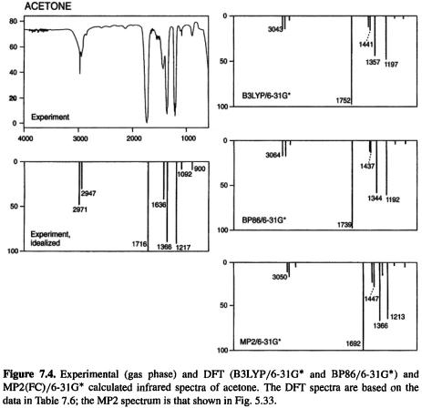
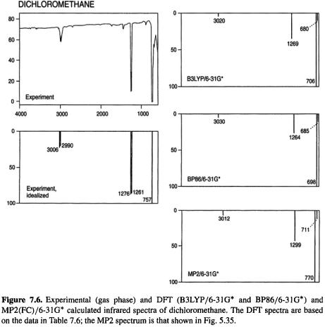
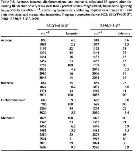
Let us examine the IR spectra of acetone, benzene, dichloromethane, and methanol, the same four compounds used in chapters 5 and 6 to illustrate calculated ab initio and semiempirical IR spectra. The DFT spectra in Figs 7.4–7.7 are based on the data in Table 7.6, and the MP2(FC)/6-31G* spectra are those used in Figs 5.33–5.36 and 6.5–6.8. The DFT methods chosen were B3LYP/6-31G* and BP86/6-31G*. The latter is used here as a substitute for pBP/DN*, which we often used for geometries and energies (for the reasons we concentrated on B3LYP and pBP, see the beginning of section 7.3.1), since as it is implemented in Spartan [47] intensities are not available from pBP/DN*. Recall (Fig. 7.3) that geometries and relative energies from B3LYP/6-31G*, B3LYP/6-311G*, and pBP/DN* were very similar; it is expected that IR spectra calculated by BP86/6-31G* and pBP/DN* will also be similar. From Figs 7.4–7.7 we see that the B3LYP/6-31G* and BP88/6-31G* spectra are very similar, and these DFT
414 Computational Chemistry
spectra are quite similar to the MP2(FC)/6-31G* spectra. The MP2 spectra simulate the experimental spectra reasonably well, but as we saw in section 5.5.3, are not (for these “routine” molecules anyway) notably superior to the HF/3-21G and HF/6-31 G* spectra.
7.3.4Properties arising from electron distribution – dipole moments, charges, bond orders, atoms-in-molecules
The theory behind calculating dipole moments, charges, and bond orders, and using atoms-in-molecules analyses, was outlined in section 5.5.4; here the results of applying DFT calculations to these will be presented.
Dipole moments
Dipole moments seem to be more sensitive to geometry than most other properties, certainly more so than is energy (of course, for certain geometries and methods, errors may tend to cancel). Another point to note is that in the perturbational DFT method (7.2.3.4c) the gradient enters the calculation only to evaluate the energy (Eq. (7.21)), after the density has converged; properties like dipole moment that are calculated from

Density Functional Calculations 415
the density will not be gradient-corrected. The gradient is applied only to energy and properties, like geometry, which are calculated from the energy. The dipole moment in such a calculation will reflect the gradient-correction only through the geometry optimization. In practice, the difference between perturbational and non-perturbational dipole moments is small [78]. Hehre [52] and Hehre and Lou [48] have provided quite extensive compilations of calculated dipole moments. These confirm that HF dipole moments tend to be larger than experimental, and show that electron correlation, through DFT or MP2, tends to lower the dipole moment, bringing it closer to the experimental value (e.g. for thiophene, from 0.80 D to 0.51 D for B3LYP; the MP2 value is 0.37 D and the experimental dipole moment is 0.55 D [48]).
Table 7.7 compares with experiment dipole moments, values calculated by B3LYP/6-31G*, pBP/DN*, by single-point B3LYP/6-31G* on AM1 geometries, and by MP2/FC/6-31G*, for 10 molecules (note that the pBP moments are not gradientcorrected, as explained above). The three DFT methods give quite similar average errors, ca. 0.1 D. Note that the smallest error, 0.09 D, is from the fast method of singlepoint B3LYP calculations on AM1 geometries, and the largest error, 0.34D, is from the most time-consuming method, MP2 all the way. The DFT dipole moments are distinctly better than ab initio (errors ca. 0.3 D, Table 5.18) and semiempirical (errors ca.
416 Computational Chemistry
0.2–0.3 D, Table 6.5) moments. None of the methods consistently gives values accurate to within 0.1 D. Dipole moments of about the same accuracy as the DFT ones in Table 7.7 (possibly a bit less accurate than the B3LYP/6-31G*//AMl ones) were obtained with single-point gradient-corrected calculations using a large basis set and geometries from perturbational gradient-corrected/6-311G**-type basis calculations. For 21 molecules the mean of the absolute deviations was 0.12D [79]. Very accurate values (mean absolute deviation 0.06–0.07 D) can be obtained with gradient-corrected DFT and very large basis sets [55].
Charges and bond orders
The theory behind these was given in section 5.5.4. Recall that these parameters are not observables and so there are no experimental, “right” values to aim for; electrostatic potential charges and Löwdin bond orders are preferred to Mulliken charges and bond orders. The effect of various computational levels on atom charges has been examined [80].

Density Functional Calculations 417
Figure 7.8 shows charges and bond orders calculated for an enolate and a protonated enone system (the same as in Fig. 6.9), using B3LYP/6-31G* and HF/3-21G. The results are qualitatively similar regardless of whether one uses B3LYP or HF, or Mulliken vs. electrostatic potential/Löwdin. This is in contrast to the results in Fig. 6.9, where there were some large differences between the semiempirical and HF/3-21G values, and even between AM1 and PM3. For example, for the protonated species using the Mulliken method, AM1 and PM3 gave the oxygen a small negative charge, ca. –0.1, but the HF/3-21G method gave it a large negative charge, –0.63; even stranger, the terminal carbon had charges of 0.09, 0.23, and -0.25 by the AM1, PM3, and HF methods. In Fig. 7.8 the biggest differences among corresponding parameters is for the electrostatic potential charges in the protonated species, where the charges on the oxygen (–0.35 and
–0.63) and on the carbonyl carbon (0.41 and 0.76) differ by a factor of about two. With both B3LYP and HF the terminal carbon of the enolate is counterintuitively assigned a bigger negative electrostatic potential charge than the oxygen, as was the case for AM1 and DFT. The calculated negative charge on the formally positive oxygen of the protonated molecule was commented on in section 6.3.4. As with the semiempirical values, bond orders are less variable here than are the charges, but even for this parameter
418 Computational Chemistry
there is one qualitative discrepancy: for the cation C/OH bond the Mulliken HF bond order is essentially single (1.18), while for the Löwdin B3LYP calculation the bond is essentially double (bond order 1.70). These results remind us that charges and bond orders are useful mainly for revealing trends, when a series of molecules, or stages along a reaction coordinate [81] are studied, all with the same methods (e.g.  and Löwdin bond orders).
Atoms-in-molecules
The atoms-in-molecules (AIM) analysis of electron density, using ab initio calculations, was considered in section 5.5.4. A comparison of AIM analysis by DFT with that by ab initio calculations by Boyd et al. showed that results from DFT and ab initio

 toward the carbon and increases the electron density in the bonding regions, compared to QCISD calculations [82].
420 Computational Chemistry
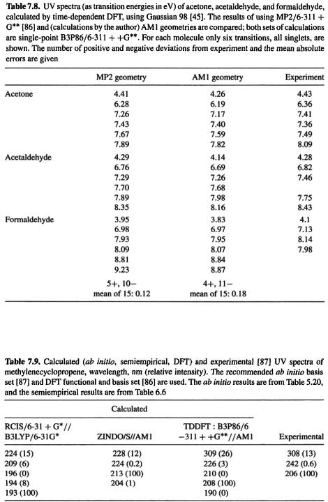
DFT is based on the time-dependent KS equations, derived from the time-dependent Schrödinger equation [84]. The implementation of time-dependent DFT (TDDFT, or time-dependent density functional response theory, TD-DFRT) in Gaussian 98 [45] has been described by Stratman et al. [85]. Wiberg et al. used this implementation to study the effect of five functional and five basis sets on the transition energies (the UV absorption wavelengths) of formaldehyde, acetaldehyde, and acetone [86]. Satisfactory results were obtained, and the energies were not strongly dependent on the functional, but B3P86 seemed to be the best and B3LYP the worst. The 6 – 311 + +G** basis was recommended. Although these workers used MP2/6-311 + G** geometries, the results in Table 7.8 indicate that AM1 geometries, which can be calculated perhaps a thousand times faster, gives transition energies that are nearly as accurate (mean absolute errors of 0.12 and 0.l8 eV, respectively). Table 7.9 compares with experiment the UV spectrum of methylenecyclopropene, calculated by ab initio, semiempirical, and DFT methods. The best of the three is the TDDFT calculation, which is the only one that reproduces the 308 nm band.
The HOMO-LUMO gap calculated with hybrid gradient-corrected functionals is approximately equal to the  UV transition of unsaturated molecules, and this could be useful in predicting UV spectra (see ionization energies and electron affinities, below).
Density Functional Calculations 421

422 Computational Chemistry
NMR spectra
As with ab initio methods (section 5.5.5), NMR shielding constants can be calculated from the variation of the energy with magnetic field and nuclear magnetic moment. The chemical shift of a nucleus is its shielding value minus that of the
TMS carbon or hydrogen nucleus (for |
or |
NMR spectra, respectively). |
The |
|
most |
accurate results are said to be |
obtained with MP2 calculations, but |
DFT |
|
is significantly better than HF [88]. |
Figure 7.9 compares with experiment |
|
||
and |
NMR spectra calculated at these levels: |
B3LYP/6-31G*//B3LYP/6-31G*, |
||
B3LYP/6-311 + G(2d,p)//B3LYP/6-31G*, B3LYP/6-311 + G(2d,p)//AMl, and HF/6-31G*//B3LYP/6-31G*. The mean absolute errors in the chemical shifts are:
B3LYP/6-31 G*//B3LYP/6-31G*
B3LYP/6-311 + G(2d, p)//B3LYP/6-31G*
B3LYP/6-311 + G(2d, p)//AM1
HF/6-31 G*//B3LYP/6-31 G*
For such a very small sample (three  and five
  atoms; the
 Hs were not included since the observed chemical shift is a weighted average) the results cannot reasonably be expected to do more than show up gross differences in accuracy, but they do suggest that for DFT NMR chemical shifts, if high accuracy is not needed there may be little point in using a bigger basis set than
 and that AM1 geometries (for normal molecules, as usual) may be as good for these spectra as B3LYP/6-31G* geometries.
Density Functional Calculations 423
Ionization energies and electron affinities
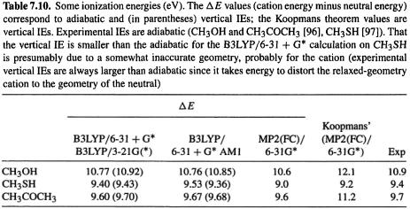
These concepts were discussed in section 5.5.5. We saw that ionization energies (ionization potentials) and electron affinities can be calculated in a straightforward way as the energy difference between a molecule and the species derived from it by loss or gain, respectively, of an electron. Using the energy of the optimized geometry of the radical cation or radical anion (in the case where the species whose IE or EA we seek is a neutral closed-shell molecule) gives the adiabatic IE or EA, while using the energy of the ionized species at the geometry of the neutral gives the vertical IE or EA. Muchall et al. have reported adiabatic and vertical ionization energies and electron affinities of eight carbenes, calculated in this way by semiempirical, ab initio, and DFT methods [91]. They recommend B3LYP/6-31 + G*//B3LYP/3-21G(*) as the method of choice for predicting first ionization energies; the use of the small 3-21G(*) basis with B3LYP for the geometry optimization is unusual – see section 5.4.2 – usually the smallest basis used with a correlated method is 6-31G*. This combination is relatively undemanding and gives accurate (largest absolute error 0.14eV) adiabatic and vertical ionization energies for the carbenes studied. Table 7.10 shows the results of applying this method to some other (non-carbene) molecules. The B3LYP/6-31 + G* energy differences are essentially the same with B3LYP/3-21G( * )and AM 1 geometries; they are good estimates of the experimental IE, are somewhat better than the ab initio MP2 energy difference values, and are considerably better than the MP2 Koopmans’ theorem (below) IBs. Of course, for unusual molecules (like the carbenes studied by Muchall et al. [91]) AM1 may not give good geometries, and for such species it would be safer to use B3LYP/3-21G(*) or B3LYP/6-31G* geometries for the single-point B3LYP/6-31 + G* calculations.
In wavefunction theory an alternative way to find IEs for removal of an electron from any molecular orbital is to invoke Koopmans’ theorem: the IE for an orbital is the negative of the orbital energy; section 5.5.5. In chapters 5 and 6 both the energy difference and the Koopmans’ theorem methods were used to calculate some IEs (Tables 5.21 and 6.7). The problem with applying Koopmans’ theorem to DFT is that in DFT proper
424 Computational Chemistry
there are no molecular orbitals, only electron density. The KS molecular orbitals (the orbitals  that make up the Slater determinant of Eq. (7.19) were, as explained in section 7.2.3.2, introduced only to provide a practical way to calculate the energy (note Eqs (7.21), (7.22), and (7.26)). There was at one time a fair amount of argument over the physical meaning, if any, of the KS orbitals. Baerends and coworkers [92] and others have suggested that the KS orbitals, like the HF orbitals, provide a good basis for qualitative discussion. Stowasser and Hoffmann showed that the KS orbitals resemble those of conventional wavefunction (extended Hückel – chapter 4 – and HF ab initio) theory in shape, symmetry, and, usually, energy order [93]. They conclude that these orbitals can indeed be treated much like the more familiar orbitals of wavefunction theory. Furthermore, they showed that although the KS orbital energy values (the eigenvalues
  from diagonalization of the DFT Fock matrix – section 7.2.3.3) are not good approximations to the ionization energies of molecular orbitals (as revealed by photoelectron spectroscopy), there is a linear relation between
  and
and  (HF). Salzner et al., too, showed that in DFT, unlike ab initio theory calculations, negative HOMO energies are not good approximations to the IE [94], but, surprisingly, HOMO-LUMO gaps from hybrid functionals agreed well with the
  UV transitions of unsaturated molecules.
Concerning electron affinities, in HF calculations the negative LUMO energy of a species M corresponds to the electron affinity not of M but rather of the anion M– [95]. However, Salzner et al. reported that the negative LUMOs from LSDA functionals gave rough estimates of EA (ca. 0.3–1.4 eV too low; gradient-corrected functionals were much worse, ca. 6eV too low) [94]. Brown et al. found that for eight medium-sized organic molecules the energy difference method using gradient-corrected functionals predicted electron affinities fairly well (average mean error less than 0.2 eV) [77].
Electronegativity, hardness, softness and the Fukui function
The idea of electronegativity was probably born about as soon as chemists suspected that the formation of chemical compounds involved electrical forces: metals and nonmetals were seen to possess opposite appetites for the “electrical fluid(s)” of eighteenth century physics. This “electrochemical dualism” is most strongly associated with Berzelius [98], and is clearly related to our qualitative notion of electronegativity as the tendency of a species to attract electrons. Parr and Yang have given a sketch of attempts to quantify the idea [99]. Electronegativity is a central notion in chemistry.
Hardness and softness as chemical concepts were apparently in the chemical literature as early as the 1950s [100], but did not become widely used till they were popularized by Pearson in 1963 [101]. In the simplest terms, the hardness of a species (atom, ion, or molecule) is a qualitative indication of how polarizable it is, i.e. how much its electron cloud is distorted in an electric field. In this sense the terms hard, and its opposite soft, were evidently suggested by D. H. Busch [101a] by analogy with the conventional use of these words to denote resistance to deformation by mechanical force. The hard/soft concept proved useful, particularly in rationalizing acid–base chemistry [102]. Thus, a proton, which cannot be distorted in an electric field (it has no electron cloud) is a very hard acid, and tends to react with hard bases. Bases in which sulfur electron pairs provide the basicity are soft, since sulfur is a big, fluffy atom, and they tend to react with soft acids. Perhaps because it was originally qualitative the hard–soft

 changes as one
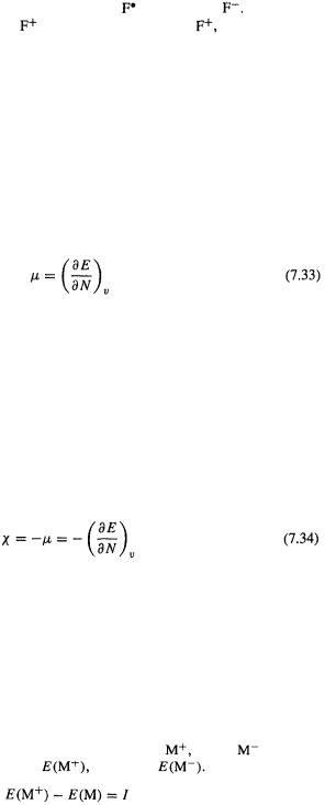
426 Computational Chemistry |
|
|
|
and then two electrons are added, giving a radical |
and an anion |
The number |
|
of electrons N we have added to |
(N is taken here as 0 for |
and is thus 1 for |
|
the atom and 2 for the anion) is integral (1,2,...), but mathematically we can consider adding continuous electronic charge N; the line through the three points is then a continuous curve and we can examine  the derivative of E with respect to N at constant nuclear charge. Ca. 1875 Willard Gibbs studied theoretically the effect on the energy of a system of a change in its composition. The derivative
  is the change in energy caused by an infinitesimal change in the number of moles n, at constant temperature and pressure; it is called the chemical potential [106]. By analogy,
 the change in energy with respect to number of added electrons at constant nuclear charge, is the electronic chemical potential (or in an understood context just the chemical potential) of an atom. For a molecule the differentiation is at constant nuclear framework, the charges and their positions being constant, i.e. constant external potential,
  (section 7.2.3.1). So for an atom, ion, or molecule
The electronic chemical potential of a molecular (including atomic or ionic) species, according to Eq. (7.33), is the infinitesimal change in energy when electronic charge is added to it. Figure 7.10 suggests that the energy will drop when charge is added to a species, at least as far as common charges (from about +3 to – 1) go, and indeed, even for fluorine’s electronegative antithesis, lithium, the energy drops along the sequence (QCISD(T)/6-311+G* gives energies of –7.23584, –7.43203, –7.45448 h, respectively). Now, since one feels intuitively that the more electronegative a species, the more its energy should drop when it acquires electrons, we suspect that there should be a link between the chemical potential and electronegativity. If we choose for convenience to make (most) electronegativities positive, then since
  is negative we might define the electronegativity
  as the negative of the electronic chemical potential:
From this viewpoint the electronegativity of a species is the drop in energy when an infinitesimal amount (infinitesimal so that it remains the same species) of electronic charge enters it. It is a measure of how hospitable an atom or ion, or a group or atoms in a molecule (section 5.5.4), is to the ingress of electronic charge, which fits in with our intuitive concept of electronegativity.
This definition of electronegativity was given in 1961[107] and later (1978) discussed in the context of DFT [108]. Equation (7.34) could be used to calculate electronegativity by fitting an empirical curve to calculated energies for, e.g.  M and
M and  and calculating the slope (gradient, first derivative) at the point of interest; however, the equation can be used to derive a simple approximate formula for electronegativity
using a three-point approximation. For consecutive species |
M and |
(constant |
|
nuclear framework), let the energies be |
E(M),and |
Then, bydefinition |
|
Density Functional Calculations 427
the ionization energy of M, and
the electron affinity of M. Adding,
So, approximating the derivative at the point corresponding to M as the change in E when N goes from 0 to 2, divided by this change in electron number, we get
i.e. using Eq. (7.34)
To use this formula one can employ experimental or calculated adiabatic (or vertical, if the species from removal or addition of an electron are not stationary points) values of I and A. This same formula (Eq. (7.35) for  was elegantly derived by Mulliken (1934) [109] using only the definitions of I and A. Consider the reactions
and
If X and Y have the same electronegativity then the energy changes of the two reactions are equal, since X and Y have the same proclivities for gaining and for losing electrons, i.e.
i.e. (I + A) for X = (I + A) for Y.
So it makes sense to define electronegativity as I + A; the factor of  (Eq. (7.35)) was said by Mulliken to be “probably better for some purposes” (possibly to make
  the arithmetic mean of I and A, an easily-grasped concept).
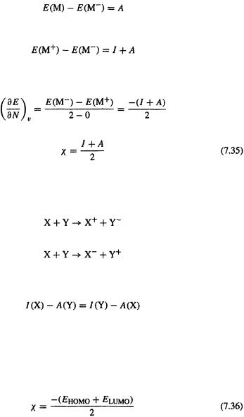
Electronegativity has also been expressed in terms of orbital energies, by taking I as the negative of the HOMO energy and A as the negative of the LUMO energy [110]. This gives
This expression has the advantage over Eq. (7.35) that one needs only the HOMO and LUMO energies of the species, which are provided by a one-pot calculation (i.e. by what is operationally a single calculation), but to use Eq. (7.35) one needs (cf. Fig. 7.10) the energy of the (N – 1)-, N- and (N + l)-electron molecules (most simply at the geometry of the molecule whose electronegativity we are calculating; cf. the Fukui functions for SCN– later in this section). How good is Eq. (7.36)?  is a fairly good approximation for the orbitals of wavefunction theory, but not for the KS
428 |
Computational Chemistry |
|
orbitals, and |
is only a very rough approximation for the KS orbitals, and |
|
for wavefunction orbitals |
of M is said to correspond to the electron affinity |
|
of |
not of M (see Ionization energies and electron affinities in section 7.3.5). So |
|
how do the results of calculations using the formula of Eq. 7.36 compare with those using Eq. (7.35)? Table 7.11 gives values of  calculated using QCISD(T)/6-311 + G* (section 5.4.3) values of I and A, which should give good values of these latter two quantities, and compares these
  values with those from HOMO/LUMO energies calculated by ab initio (MP2(FC)/6-31G*) and by DFT (B3LYP/6-31G*). For the two cations the agreement between the three ways of calculating
  is good; for the other species it is erratic or bad, although the trends are the same for the three methods within a given family (hardness decreases from cation to radical to anion). There seems little doubt that Eq. (7.35) is the sounder way to calculate electronegativity. An exposition of the concept of electronegativity as the (negative) average of the HOMO and LUMO energies, and the chemical potential
 as lying at the midpoint of the HOMO/LUMO gap, has been given by Pearson [110].
Chemical hardness and softness are much newer ideas than electronegativity, and they were quantified only fairly recently. Parr and Pearson (1983) proposed to identify the curvature (i.e. the second derivative) of the E vs. N graph (e.g. Fig. 7.10) with hardness,  [111]. This accords with the qualitative idea of hardness as resistance to deformation, which itself accommodates the concept of a hard molecule as resisting polarization – not being readily deformed in an electric field: if we choose to define hardness as the curvature of the E vs. N graph, then
where  and
and  are introduced from Eqs (7.33) and (7.34). The hardness of a species is then the amount by which its electronegativity – its ability to accept electrons – decreases when an infinitesimal amount of electronic charge is added to it. Intuitively, a hard molecule is like a rigid container that does not yield as electrons are forced in, so the pressure (analogous to the electron density) inside builds up, resisting the ingress of more electrons. A soft molecule may be likened to a balloon that can expand as it acquires electrons, so that the ability to accept still more electrons is not so seriously compromised. Softness is the reciprocal of hardness:
and qualitatively, of course, it is the opposite in all ways.
To approximate hardness by I and A (cf. the approximation of electronegativity by Eq. (7.35)), we approximate the  curve (cf. Fig. 7.10) by a general quadratic (it looks like a quadratic):

Density Functional Calculations 429
430 Computational Chemistry |
|
|
|
We will now let M denote any atom or molecule, and |
and |
the species formed |
|
by removal or addition of an electron. |
|
|
|
E(M) corresponds to N = 1 and |
corresponds to N = 2, |
so substituting into |
|
our quadratic equation
and
and so
Since 
i.e.
Actually, the hardness is commonly defined as half the curvature of the E vs. N graph, giving
and from Eq. (7.37)
The one-half factor is [110] to bring into line with Eq. (7.35), where this factor arises naturally in applying the three-point approximation and the definitions of I and A to the rigorous Gibbs equation (Eq. (7.33)) for electronic chemical potential.
Electronegativity has also been expressed in terms of orbital energies, by taking I as the negative of the HOMO energy and A as the negative of the LUMO energy [110]. This gives
Like the analogous expression for electronegativity (Eq. (7.36)), this requires only a “one-pot” calculation, of the HOMO and LUMO. Much of what was said about Eq. (7.36) applies to Eq. (7.42). Table 7.11 gives values of calculated analogously to the
  values discussed above. The HOMO/LUMO hardness values are in even worse agreement with the I/A ones than are the HOMO/LUMO electronegativity values with the I/A values (the zero values for the HOMO/LUMO-calculated
  of the radicals values arise from taking the half-occupied orbital (semioccupied MO, SOMO) as both HOMO and LUMO). The orbital view of hardness as the HOMO/LUMO gap is discussed by Pearson, who also reviews the principle of maximum hardness, according to which in a chemical reaction hardness and the HOMO/LUMO gap tend to increase,

Density Functional Calculations 431
potential energy surface relative minima represent species of relative maximum hardness, and transition states are species of relative minimum hardness [110]. In recent papers these general ideas about hardness are expounded [112] and the reciprocal concept of softness is used (with the Fukui function) to rationalize some cycloaddition reactions [113].
The Fukui function (the frontier function) was defined by Parr and Yang [104] as
This says that  is the functional derivative (section 7.2.3.2, The Kohn–Sham equations) of the chemical potential with respect to the external potential (i.e. the potential caused by the nuclear framework), at constant electron number; and that it is also the derivative of the electron density with respect to electron number at constant external potential. The second equality shows
  to be the sensitivity of
  to a change in N, at constant geometry. A change in electron density should be primarily electron withdrawal from or addition to the HOMO or LUMO, the frontier orbitals of Fukui [114], hence the name bestowed on the function by Parr and Yang. Since
  varies from point to point in a molecule, so does the Fukui function. Parr and Yang argue that a large value of
  at a site favors reactivity at that site, but to apply the concept to specific reactions they define three Fukui functions (“condensed Fukui functions” [80]):
The three functions  and
and  refer to an electrophile, a nucleophile, and a radical. They are the sensitivity, to a small change in the number of electrons, of the electron density in the LUMO, the HOMO, and in a kind of average HOMO/LUMO half-occupied orbital. Practical implementations of these condensed Fukui functions are the “condensed-to-atom” forms of Yang and Mortier [115]:
Here |
is the electron population (not the charge) on atom k, etc. (see below). |
||
Note that |
is just the average of |
and |
The condensed Fukui functions measure |
the sensitivity to a small change in the number of electrons of the electron density at atom k in the LUMO  in the HOMO
 and in a kind of intermediate orbital
  they provide an indication of the reactivity of atom k as an electrophile (reactivity toward nucleophiles), as a nucleophile (reactivity toward electrophiles), and as a free radical (reactivity toward radicals).
The easiest way to see how these formulas can be used is to give an example. Let us calculate  for the anion
  We shall calculate
  and
and  to get an idea of the nucleophilic power of the S, C, and N atoms in this molecule. We need the electron population q on each atom or, what gives us the same information, the
432 Computational Chemistry
charge on each atom (for an atom in a molecule, electron population + charge =
atomic number). We perform the calculations for the N-electron species |
and |
|||
the (N – l)-electron species |
If we were interested in the nucleophilic power |
|||
of the atoms in a neutral molecule M, then to get |
we would calculate the electron |
|||
populations or charges on the atoms in M and in |
and for the electrophilic power of |
|||
the atoms in neutral M, to get |
we calculate the electron populations or charges on |
|||
the atoms in M and |
The calculations are performed for the two species at the same |
|||
geometry. In introducing the condensed Fukui function, Yang and Mortier [115] used for each pair of species a single “standard” (presumably essentially average) geometry, with accepted, reasonable bond lengths and angles, and other workers do not specify
whether they use for, say, M and |
the neutral or the cation geometry. We will |
||
adopt the convention that for a calculation on |
both geometries |
||
will be those of |
the species of interest to us; |
this avoids the problem of trying |
|
to do a geometry optimization on a species that may not be a stationary point on the potential energy surface (assuming that  is itself a stationary point – one will rarely be interested in something that is not), a situation that arises particularly for some
anions. |
|
|
|
Charges and electron populations from calculations on |
and |
(and on |
|
and |
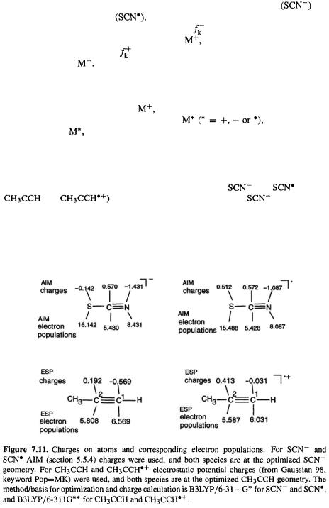
are shown in Fig. 7.11. The anion |
|
was optimized |
and then the AIM (section 5.5.4) electron population/charges were calculated (the AIM calculations were done with G98 using the keywords AIM = Charge). An AIM calculation was then done on the radical at the anion geometry. The optimization and both

Density Functional Calculations 433
AIM calculations used the B3LYP/6-31 + G* method/basis (results for charges other than AIM and other methods/basis sets are shown shortly).
The condensed Fukui functions may now be calculated (see Fig. 7.11):
This indicates that in  the order of nucleophilicity is
  (which is what any chemist would expect). Sulfur is the softest atom here, and carbon the hardest. The results of such a calculation vary somewhat with the method/basis (e.g. HF/6-31G*, MP2/6-31G*, etc.), and especially with the way the charges/electron populations are calculated. Here are the
  functions from the use of electrostatic potential charges (the G98 keyword Pop=MK was used) again using B3LYP/6-31 + G*:
In this case the conclusions are unaffected.
In an extensive study, Geerlings et al. [80] showed that with AIM charges semiquantitatively similar results are obtained with a variety of correlation methods (HF, MP2, QCISD, and five DFT functionas), using bases similar to 6-31G*. The biggest deviation from QCISD (section 5.4.3; QCISD was taken as the most reliable of the methods used) was shown by MP2. For example, for  all correlation methods except MP2 gave O a bigger
  than C. If we disregarded the MP2 result as anomalous, this could be interpreted as indicating that the O is more nucleophilic than the C. Actually, in standard organic syntheses enolates usually react preferentially at the carbon, but the ratio of C:O nucleophilic attack can vary considerably with the particular enolate, the electrophile, and the solvent. To complicate things even more, the nucleophile is not always just the simple enolate: an ion pair or even aggregates of ion pairs may be involved [116]. Even for the case of an unencumbered enolate, the atom with the biggest
 (the softest atom) cannot be assumed to be the strongest nucleophilic center, because, as
  and
and  point out in their study [117] of enolates using the Fukui function, one consequence of the HSAB principle is that an electrophile tends to react with a nucleophilic center of similar softness (soft acids prefer soft bases, etc.), not necessarily with the softest nucleophilic center. Thus, for the reaction of
with the electrophile one might calculate, for  and
and 
and for The would be expected (in the absence of complica- tions!) to bond to the atom (C or O) whose  value was closest to its
 value. A study of the ethyl acetoacetate enolate using these and other concepts has been reported by Geerlings and coworkers [118]. This approach, which is applicable to any ambident species, is further illustrated below by the reaction of HNC with alkynes.
434 Computational Chemistry
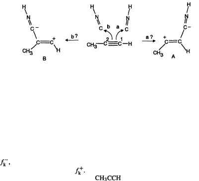
In a study of the reaction of alkynes with hydrogen isocyanide the condensed Fukui function was combined with the overall or global softness to try to rationalize the regioselectivity of attack on the triple bond [113]:
This reaction involves electrophilic attack by HNC on the alkyne, to give a zwitterion which reacts further. Can our concepts be used to predict which alkyne atom,  or
or  (using the designations of Nguyen et al. [113]) will be attacked – will the products be formed primarily through A or through B? Nguyen et al. approached this problem by first showing that the reaction is indeed electrophilic attack of HNC (i.e. acting as an electrophile) on the alkyne (acting as a nucleophile): the HOMO(alkyne)/LUMO(HNC) interaction has a smaller energy gap than the HOMO(HNC)/LUMO(alkyne) interaction. They then calculated the local softness or condensed softness parameters (not quite the same as the condensed-to-atoms parameters of Eqs (7.45) that we saw above; see below) of
 and
and  of the alkyne and the C of HNC. For
  and
and  of the alkyne the softness as a nucleophile, i.e. softness toward electrophiles, was calculated, with the aid
of |
and for the HNC C softness as an electrophile, i.e. softness toward nucleophiles, |
|
was calculated, with the aid of |
|
|
|
Illustrating how the calculations for |
may be done: |
(1)Optimize the structure of  and calculate its atom charges (and energy).
(2)Use the optimized geometry of  for a single-point (same geometry) calculation of the charges (and energy) for
  Steps (1) and (2) enable calculation of
(3)Use the optimized geometry of  for a single-point calculation of the energy of the anion
  (This is a radical anion).
Steps (1), (2), and (3) enable us to calculate the global softness (the softness of the molecule as a whole) of This is done by calculating the vertical ionization energy and electron affinity as energy differences, then calculating the global softness as the reciprocal of global hardness. From Eq. (7.38) this is
  or
or  2/(I – E), depending on whether we define hardness according to Eq. (7.39) or (7.40). Nguyen et al. use
  i.e they take hardness as
  rather than
  The local softness of any atom of interest may now be calculated by multiplying
  for that atom by
  Let us look at actual numbers. The
  B3LYP/6-311G** basis set and electrostatic potential charges (with the Gaussian keyword Pop=MK) were used. These gave the charges (and thus electron
Density Functional Calculations 435
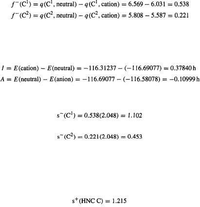
populations) shown in Fig. 7.11. From these populations,
The vertical ionization energy and vertical electron affinity are (here ZPEs have not been taken into account, as they should nearly cancel; in any case the significance of a calculated ZPE for the cation or anion at the geometry of the neutral is questionable, since the former two vertical species are not stationary points):
The softness is then  So the local softness of the two carbons as nucleophiles (softness toward electrophiles) is
and
(Nguyen et al. report 1.096 and 0.460).
Since electron population is a pure number and global softness has the units of reciprocal energy, local softness logically has these units too, but the practice is to simply state that all these terms are in “atomic units”.
Now consider analogous calculations on the HNC C, but for local softness as an electrophile (softness toward nucleophiles), using  These calculations gave
To predict which of the two alkyne carbons,  or
or  HNC will preferentially attack, one now invokes the “local HSAB principle” [119], which says that interaction is favored between electrophile/nucleophile (or radical/radical) of most nearly equal softness. The HNC carbon softness of 1.215 is closer to the softness of
  (1.102) than that of
  (0.453) of the alkyne, so this method predicts that in the reaction scheme above the HNC attacks
  in preference to
  i.e. that reaction should occur mainly by the zwitterion A. This prediction agreed with that from the more fundamental approach of calculating the activation energies as the difference of transition state and reactant energies. This kind of analysis worked for
  and
and  substituents on the alkyne, but not for –F.
The concepts of hardness, softness, and of frontier orbitals, with which latter the Fukui function is closely connected, have been severely criticized [103, 120]. It is also true that in some cases the results predicted using these methods can also be understood in terms of more traditional chemical concepts. Thus, in the alkyne–HNC reaction, resonance theory leads one to suspect that the zwitterion A, with the positive charge formally on the more substituted carbon, will be favored over B. Indeed, AM1,
 DFT calculations all show A to be of lower energy than B.