


Introduction to Quantum Mechanics 91
4.2.6 The wave mechanical atom and the Schrödinger equation
The Bohr approach works well for hydrogen-like atoms, atoms with one electron: hydrogen, singly-ionized helium, doubly-ionized lithium, etc. However, it showed many deficiencies for other atoms, which is to say, almost all atoms of interest other than hydrogen. The problems with the Bohr atom for these cases were described below.
(1) There were lines in the spectra corresponding to transitions other than simply between two n values (cf. Eq. (4.14)). This was rationalized by Sommerfeld in 1915, by the hypothesis of elliptical rather than circular orbits, which essentially introduced a new quantum number k, a measure of the eccentricity of the elliptical orbit. Electrons could have the same n but different ks, increasing the variety of possible electronic transitions; k is related to what we now call the azimuthal quantum number, 
(2) There were lines in the spectra of the alkali metals that were not accounted for by the quantum numbers n and k. In 1925 Goudsmit and Uhlenbeck showed that these could be explained by assuming that the electron spins on an axis; the magnetic field generated by this spin around an axis could reinforce or oppose the field generated by the orbital motion of the electron around the nucleus. Thus for each n and k there are two closely-spaced “magnetic levels,” making possible new, closely-spaced spectral lines. The spin quantum number,  or
or  was introduced to account for spin.
(3) There were new lines in atomic spectra in the presence of an external magnetic field (not to be confused with the fields generated by the electron itself). This Zeeman effect (1896) was accounted for by the hypothesis that the electron orbital plane can take up only a limited number of orientations, each with a different energy, with respect to the external field. Each orientation was associated with a magnetic quantum number
 (often designated m) = –l, –(l – 1), …, (l – 1), l. Thus in an external magnetic field the numbers n, k (later l) and
  are insufficient to describe the energy of an electron and new transitions, invoking
  are possible.
The only quantum number that flows naturally from the Bohr approach is the principal quantum number, n; the azimuthal quantum number l (a modified k), the spin quantum number  and the magnetic quantum number
  are all ad hoc, improvised to meet an experimental reality. Why should electrons move in elliptical orbits that depend on the principal quantum number n? Why should electrons spin, with only two values for this spin? Why should the orbital plane of the electron take up with respect to an external magnetic field only certain orientations, which depend on the azimuthal quantum number? All four quantum numbers should follow naturally from a satisfying theory of the behaviour of electrons in atoms.
The limitations of the Bohr theory arise because it does not reflect a fundamental facet of nature, namely the fact that particles possess wave properties. These limitations were transcended by the wave mechanics of Schrödinger,16 when he devised his famous equation in 1926 [ 12,13]. Actually, the year before the Schrödinger equation was
16Erwin Schrödinger, born Vienna, 1887. Ph.D. University of Vienna. Professor Stuttgart, Berlin, Graz (Austria), School for Advanced Studies Dublin, Vienna. Nobel prize in physics 1933 (shared with Dirac). Died Vienna, 1961.

92 Computational Chemistry
published, Heisenberg17 published his matrix mechanics approach to calculating atomic (and in principle molecular) properties. The matrix approach is at bottom equivalent to Schrödinger’s use of differential equations, but the latter has appealed to chemists more because, like physicists of the time, they were unfamiliar with matrices (section 4.3.3), and because the wave approach lends itself to a physical picture of atoms and molecules while manipulating matrices perhaps tends to resemble numerology. Matrix mechanics and wave mechanics are usually said to mark the birth of quantum mechanics (1925, 1926), as distinct from quantum theory (1900). We can think of quantum mechanics as the rules and equations used to calculate the properties of molecules, atoms, and subatomic particles.
Wave mechanics grew from the work of de Broglie,18 who in 1923 was led to this “wave-particle duality” by his ability to deduce the Wien blackbody equation (section 4.2.1) by treating light as a collection of particles (light quanta) analogous to an ideal gas [14]. This suggested to de Broglie that light (traditionally considered a wave motion) and the atoms of an ideal gas were actually not fundamentally different. He derived a relationship between the wavelength of a particle and its momentum, by using the time-dilation principle of special relativity, and also from an analogy between optics and mechanics. The reasoning below, while less profound than de Broglie’s, may be more accessible. From the special theory of relativity, the relation between the energy of a photon and its mass is
where c is the velocity of light. From the Planck equation (4.3) for the emission and absorption of radiation, the energy  of a photon may be equated with the energy change
  of an oscillator, and we may write
From Eqs (4.15) and (4.16)
Since  Eq. (4.17) can be written
and because the product of mass and velocity is momentum, Eq. (4.18) can be written
relating the momentum of a photon (in its particle aspect) to its wavelength (in its wave aspect). If Eq. (4.19) can be generalized to any particle, then we have
I7Werner Heisenberg, born Würzburg, Germany, 1901. Ph.D. Munich, 1923. Professor, Leipzig University, Max Planck Institute. Nobel Prize 1932 for his famous uncertainty principle of 1927. Director of the German atomic bomb/reactor project 1939–1945. Held various scientific administrative positions in postwar (Western) Germany 1945–1970. Died Munich 1976.
18Louis de Broglie, born Dieppe, 1892. Ph.D. University of Paris. Professor Sorbonne, Institut Henri Poincaré (Paris), Nobel prize in physics 1929. Died Paris, 1987.

Introduction to Quantum Mechanics 93
relating the momentum of a particle to its wavelength; this is the de Broglie equation.
If a particle has wave properties it should describable by somehow combining the de Broglie equation and a classical wave equation. A highly developed nineteenth century mathematical theory of waves was at Schrödinger’s disposal, and the union of a classical wave equation with Eq. (4,20) was one of the ways that he derived his wave equation. Actually, it is said that the Schrödinger equation cannot actually be derived, but is rather a postulate of quantum mechanics that can only be justified by the fact that it works [15]; this fine philosophical point will not be pursued here. Of his three approaches [15], Schrödinger’s simplest is outlined here. A standing wave (one with fixed ends like a vibrating string or a sound wave in a flute) whose amplitude varies with time and with the distance from the ends is described by
where f (x) is the amplitude of the wave, x is the distance from some chosen origin, and  is the wavelength. From Eq. (4.20):
where  is the wavelength of particle of mass m and velocity
  Identifying the wave with a particle and substituting for
  from (4.22) into (4.21):
Since the total energy of the particle is the sum of its kinetic and potential energies:
where E is the total energy of the particle, and V is the potential energy (the usual symbol), i.e.
Substituting Eq. (4.25) for  into Eq. (4.23):
where f (x) is the amplitude of the particle/wave at a distance  from some chosen origin, m is the mass of the particle, E is the total energy (kinetic + potential) of the particle, and V is the potential energy of the particle (possibly a function of x). This is the Schrödinger equation for one-dimensional (1D) motion along the spatial coordinate x. It is usually written
94 Computational Chemistry
where  is the amplitude of the particle/wave at a distance x from some chosen origin. The 1D Schrödinger equation is easily elevated to 3D status by replacing the 1D operator
  by its 3D analogue
 is the Laplacian operator “del squared.” Replacing
  by
by  Eq. (4.27) becomes
This is a common way of writing the Schrödinger equation. It relates the amplitude  of the particle/wave to the mass m of the particle, its total energy E and its potential energy V. The meaning of
  itself is unknown [2] but the currently popular interpretation of
  due to Born (section 2.3) and Pauli19 is that it is proportional to the probability of finding the particle near a point P(x, y, z) (recall that
  is a function of x, y, z):
The probability of finding the particle in an infinitesimal cube of sides dx, dy, dz is  dx dy dz, and the probability of finding the particle somewhere in a volume V is the integral over that volume of
  with respect to dx, dy, dz (a triple integral);
  is thus a probability density function, with units of probability per unit volume. Born’s interpretation was in terms of the probability of a particular state, Pauli’s the chemist’s usual view, that of a particular location.
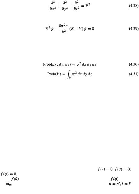
The Schrödinger equation overcame the limitations of the Bohr approach (see the beginning of section 4.2.6): the quantum numbers follow naturally from it (actually the spin quantum number ms requires a relativistic form of the Schrödinger equation, the Dirac equation, and electron “spin” is apparently not really due to the particle spinning like a top). The Schrödinger equation can be solved in an exact analytical way only for one-electron systems like the hydrogen atom, the helium monocation and the hydrogen molecule ion, but the mathematical approach is complicated and of no great relevance to the application of this equation to the study of serious molecules. However a brief account of the results for hydrogen-like atoms is in order.
The standard approach to solving the Schrödinger equation for hydrogen-like atoms involves transforming it from Cartesian (x, y, z) to polar coordinates  since these accord more naturally with the spherical symmetry of the system. This makes it
possible to separate the equation into three simpler equations, |
and |
|
|
Solution of the f(r) equation gives rise to the n quantum number, solution |
|
of the |
equation to the l quantum number, and solution of the |
equation to |
the |
(often simply called m) quantum number. For each specific |
and |
19Wolfgang Pauli, born Vienna, 1900. Ph.D. Munich 1921. Professor Hamburg, Zurich, Princeton, Zurich. Best known for the Pauli exclusion principle. Nobel Prize 1945. Died Zurich 1958.