


Introduction to Quantum Mechanics 133
The results of this charge calculation are summarized in Fig. 4.24; the negative charge on the exocyclic carbon and the positive charges on the ring carbons are in accord with the resonance picture (Fig. 4.24), which invokes a contribution from the aromatic cyclopropenyl cation [49]. Note that the charges sum to (essentially) zero, as they must for a neutral molecule (the hydrogens, which actually also carry charges, have been excluded from consideration here). A high-level calculation places a total charge (carbon plus hydrogen) – albeit defined in a different way – of –0.37 on the  group and +0.37 on the ring (cf. –0.487 and +0.487 for the exocyclic carbon and the ring carbons in the SHM calculation).
4.3.6 Strengths and weaknesses of the SHM
Strengths
The SHM has been extensively used to correlate, rationalize, and predict many chemical phenomena, having been applied with surprising success to dipole moments, esr spectra, bond lengths, redox potentials, ionization potentials, UV and IR spectra, aromaticity, acidity/basicity, and reactivity, and specialized books on the SHM should be consulted for details [21]. The method will probably give some insight into any phenomenon that involves predominantly the  electron systems of conjugated molecules. The SHM may have been underrated [50] and reports of its death are probably exaggerated. However, the SHM is not used very much in research nowadays, partly because more

134 Computational Chemistry
sophisticated  electron approaches like the PPP method (section 6.2.2) are available, but mainly because of the phenomenal success of all-valence-electron SE methods (chapter 6), which are applicable to quite large molecules, and of the increasing power of all-electron ab initio (chapter 5) and DFT (chapter 7) methods.
Weaknesses
The defects of the SHM arise from the fact that it treats only  electrons, and these only very approximately. The basic Hückel method described here has been augmented in an attempt to handle non
 substituents, e.g. alkyl groups, halogen groups, etc., and heteroatoms instead of carbon. This has been done by treating the substituents as
centers and embodying empirically altered values of |
and |
so that in the Fock |
matrix values other than –1 and 0 appear. However, |
the values of these modified |
|
parameters that have been employed vary considerably [51], which tends to diminish one’s confidence in their reliability.
The approximations in the SHM are its peremptory treatment of the overlap integrals S (section 4.3.4, discussion in connection with Eqs (4.55)), its drastic truncation of the possible values of the Fock matrix elements into just  and 0 (section 4.3.4, discussion in connection with Eqs (4.61)), its complete neglect of electron spin, and its glossing over (although not exactly ignoring) interelectronic repulsion by incorporating this into the
 and
and  parameters.
The overlap integrals S are divided into just two classes:
 or 0
or 0
depending on whether the orbitals on the atoms i and j are on the same or different atoms. This approximation, as explained earlier, reduces the matrix form of the secular equations to standard eigenvalue form  (Eq. (4.59)), so that the Fock matrix can (after giving its elements numerical values) be diagonalized without further ado (the ado is explained in section 4.3.7, in connection with the extended Hückel method). In the older determinant, as opposed to matrix, treatment (section 4.3.7), the approximation greatly simplifies the determinants. In fact, however, the overlap integral between
adjacent carbon p orbitals is ca. 0.24 [52]. |
|
Setting the Fock matrix elements equal to just |
and 0. Setting |
|
or 0 |
depending on whether the orbitals on the atoms i and j are on the same, adjacent or further-removed atoms is an approximation, because all the  terms are not the same, and all the adjacent-atom
  terms are not the same either; these energies depend on the environment of the atom in the molecule; for example, atoms in the middle of a conjugated chain should have different
  and
and  parameters than ones at the end of the chain. Of course, this approximation simplifies the Fock matrix (or the determinant in the old determinant method, section 4.3.7).
The neglect of electron spin and the deficient treatment of interelectronic repulsion is obvious. In the usual derivation (section 4.3.4): in Eq. (4.40) the integration is carried out with respect to only spatial coordinates (ignoring spin coordinates; contrast ab initio
Introduction to Quantum Mechanics 135
theory, section 5.2), and in calculating  energies (section 4.3.5) we simply took the sum of the number of electrons in each occupied MO times the energy level of the MO. However, the energy of an MO is the energy of an electron in the MO moving in the force field of the nuclei and all the other electrons (as pointed out in section 4.3.4, in explaining the matrices of Eqs (4.55)). If we calculate the total electronic energy by simply summing MO energies times occupancy numbers, we are assuming, wrongly, that the electron energies are independent of one another, i.e. that the electrons do not interact. An energy calculated in this way is said to be a sum of one-electron energies. The resonance energies calculated by the SHM can thus be only very rough, unless the errors tend to cancel in the subtraction step, which in fact probably occurs to some extent (this is presumably why the method of Hess and Schaad for calculating resonance energies works so well [50]). The neglect of electron repulsion and spin in the usual derivation of the SHM is discussed in Ref. [30].
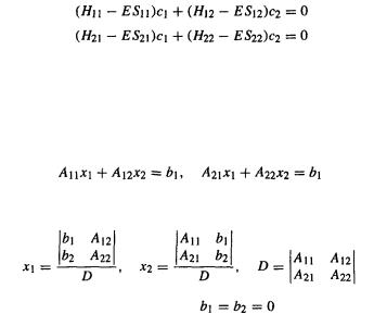
4.3.7The determinant method of calculating the Hückel c’s and energy levels
An older method of obtaining the coefficients and energy levels from the secular equations (Eqs (4.49) for a two-basis-function system) utilizes determinants rather than matrices. The method is much more cumbersome than the matrix diagonalization approach of section 4.3.4, but in the absence of cheap, readily-available computers (matrix diagonalization is easily handled by a personal computer) its erstwhile employment may be forgiven. It is outlined here because traditional presentations of the SHM [21] use it.
Consider again the secular equations (4.49):
By considering the requirements for nonzero values of  and
and  we can find how to calculate the c’s and the MO energies (since the coefficients are weighting factors that determine how much each basis function contributes to the MO, zero c’s would mean no contributions from the basis functions and hence no MOs; that would not be much of a molecule). Consider the system of linear equations
Using determinants:
where D is the determinant of the system. If equations), then in the equations for  and
and 
(the situation in the secular the numerator is zero, and so 

136 |
Computational Chemistry |
|
|
and |
The only way that |
and |
can be nonzero in this case is that the |
determinant of the system be zero, i.e.
for then  and
and  and 0/0 can have any finite value; mathematicians call it indeterminate. This is easy to see:
which is true for any finite value of 
So for the secular equations the requirement that the c’s be nonzero is that the determinant of the system be zero:
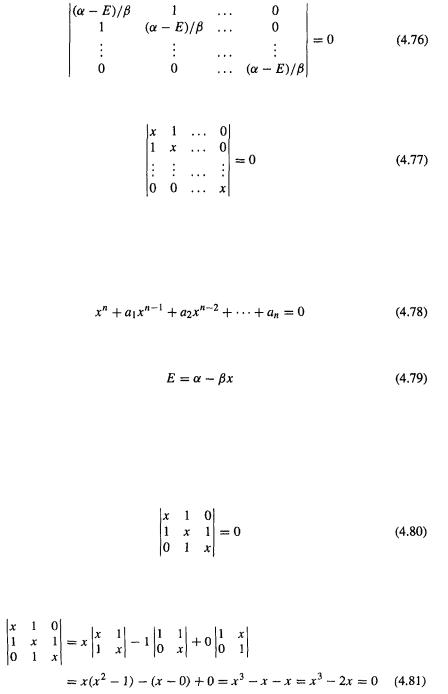
Equation (4.72) can be generalized to n basis functions (cf. the matrix of Eq. (4.62)):
If we invoke the SHM simplification of orthogonality of the S integrals (pp. 37–39), then  and
and  and Eq. (4.75) becomes
Substituting  and 0 for the appropriate H’s (p. 39) we get
The diagonal |
terms will always be – E, but the placement of and 0 will depend |
on which i, j |
terms are adjacent and which are further-removed, which depends on the |
numbering system chosen (see below). Since multiplying or dividing a determinant by a number is equivalent to multiplying or dividing the elements of one row or column
Introduction to Quantum Mechanics 137
by that number (section 4.3.3), multiplying both sides of Eq. (4.75) by  n times, i.e. by
  gives
gives
Finally, if we define  we get
The diagonal terms are always x but the off-diagonal terms, 1 for adjacent and 0 for nonadjacent orbital pairs, depend on the numbering (which does not affect the results: Fig. 4.25). Any specific determinant of the type in Eq. (4.77) can be expanded into a polynomial of order n (where the determinant is of order n × n), making Eq. (4.77) yield the polynomial equation:
The polynomial can be solved for x and then the energy levels can be found from  from
from
The coefficients can then be calculated from the energy levels by substituting the E’s into one of the secular equations, finding the ratio of the c’s, and normalizing to get the actual c’s. An example will indicate how the determinant method can be implemented.
Consider the propenyl system. In the secular determinant the i, i-type interactions will be represented by x, adjacent i, j-type interactions by 1, and nonadjacent i, j-type interactions by 0. For the determinantal equation we can write (Fig. 4.25)
(Compare this with the Fock matrix for the propenyl system). Solving this equation (see section 4.3.3):

138 Computational Chemistry
This cubic can be factored (but in general polynomial equations require numerical approximation methods):
so |
and |
or |
From |
and |
|
|
leads to |
|
|
leads to |
|
|
leads to |
|
So we get the same energy levels as from matrix diagonalization 
To find the coefficients we substitute the energy levels into the secular equations; for the propenyl system these are, projecting from the secular equations for a two-orbital system, Eqs (4.49):
These can be simplified (Eqs (4.57) and (4.61)) to
For the energy level  (MO level 1,
  substituting into the first secular equation we get
so

Introduction to Quantum Mechanics 139
(Recall the  notation;
  is the coefficient for atom 1 in
 is the coefficient for atom 2 in
  etc.) Substituting
  into the second secular equation we get
We now have the relative values of the c’s:
To find the actual values of the c’s, we utilize the fact that the MO (we are talking about MO level 1,  must be normalized:
Now, from the LCAO method
Therefore
So from Eq. (4.87), and recalling that in the SHM we pretend that the basis functions  are orthonormal, i.e. that
  we get
Using the ratios of the c’s from Eq. (4.84):
i.e.
and so
By substituting into the secular equations (4.83) the E values for  and
and  we could find the ratios of the c’s for
 and
and and with the aid of the orthonormalization equation analogous to Eq. (4.88) we could get the actual values of
  and
and 
 and
and  Although this somewhat clumsy way of finding the c’s from the energy levels was streamlined (see, e.g. [21d]), the determinant method has been replaced by matrix diagonalization implemented in a computer program.