

140 Computational Chemistry
4.4THE EXTENDED HÜCKEL METHOD
4.4.1Theory
In the SHM, as in all modern MO methods, a Fock matrix is diagonalized to give coefficients (which with the basis set give the wavefunctions of the MOs) and energy levels (i.e. MO energies). The SHM and the extended Hückel method (EHM, extended Hückel theory, EHT) differ in how the elements of the Fock matrix are obtained and how the overlap matrix is treated. The EHM was popularized and widely applied by Hoffmann28 [53], although earlier work using the approach had been done by Wolfsberg and Helmholz [54], We now compare point by point the SHM and the EHM.
Simple Hückel method
(1) Basis set is limited to p orbitals. Each element of the Fock matrix H is an integral that represents an interaction between two orbitals. The orbitals are in almost all cases a set of p orbitals (usually carbon 2p) supplied by an  framework, with the p orbital axes parallel to one another and perpendicular to the plane of the framework. In other words, the set of basis orbitals – the basis set – is limited (in the great majority of cases) to
  orbitals (taking the framework plane, i.e. the molecular plane, to be the xy plane).
(2) Orbital interaction energies are limited to and 0. The Fock matrix orbital interactions are limited to
  and 0, depending on whether the
  interaction is, respectively i, i, adjacent, or further-removed. The value of
  does not vary smoothly with the separation of the orbitals, although logically it should decrease continuously to zero as the separation increases.
(3) Fock matrix elements are not actually calculated. The Fock matrix elements are not any definite physical quantities, but rather energy levels relative to  in units of
  making them 0 or –1. One can try to estimate
 and
and  but the SHM does not define them quantitatively.
(4) Overlap integrals are limited to 1 or 0. We pretend that the overlap matrix S is a unit matrix, by setting  This enables us to simplify
  (Eq. (4.54)) to the standard eigenvalue form
  (Eq. (4.59)) and so
  which is the same as saying that the SHM Fock matrix is directly diagonalized to give the c’s and
Now compare these four points with the corresponding features of the EHM.
Extended Hückel method
(1) All valence s and p orbitals are used in the basis set. As in the SHM each element of the Fock matrix is an integral representing an interaction between two orbitals; however, in the EHM the basis set is not just a set of orbitals but rather the set of valenceshell orbitals of each atom in the molecule (the derivation of the secular equations
28 Roald Hoffmann, born Zloczow, Poland, 1937. Ph.D. Harvard, 1962, Professor, Cornell. Nobel prize 1981 (shared with Kenichi Fukui; section 7.3.5) for work with organic chemist Robert B. Woodward, showing how the symmetry of molecular orbitals influences the course of chemical reactions (the Woodward– Hoffmann rules or the conservation of orbital symmetry). Main exponent of the extended Hückel method. He has written poetry, and several popular books on chemistry.
Introduction to Quantum Mechanics 141
says nothing about what kinds of orbitals we are considering). Thus each hydrogen atom contributes a 1s orbital to the basis set and each carbon atom a 2s and three 2p orbitals. Lithium and beryllium, although they have no 2p electrons, are assigned a 2s and three 2p orbitals (experience shows that this works better than omitting these basis functions) so the atoms from lithium to fluorine each contribute a 2s and three 2p orbitals. A basis set like this, which uses the normal valence orbitals of atoms, is called a minimal valence basis set.
(2)Orbital interaction energies are calculated and vary smoothly with geometry.
The EHM Fock matrix orbital interactions  are calculated in a way that depends on the distance apart of the orbitals, so their values vary smoothly with orbital separation.
(3)Fock matrix elements are actually calculated. The EHM Fock matrix elements are calculated from well-defined physical quantities (ionization energies) with the aid of well-defined mathematical functions (overlap integrals), and so are closely related to ionization energies and have definite quantitative values.
(4)Overlap integrals are actually calculated. We do not in effect ignore the overlap
matrix, i.e. we do not set it equal to a unit matrix. Instead, the elements of the overlap
matrix are calculated, each  depending on the distance apart of the atoms i and j, which has the important consequence that the S values depend on the geometry of the
molecule. Since S is not taken as a unit matrix, we cannot go directly from  to
to  and thus we cannot simply diagonalize the EHM Fock to get the c’s and
These four points are elaborated on below.
(1) Use of a minimal valence basis set in the EHM is more realistic than treating just the  orbitals, since all the valence electrons in a molecule are likely to be involved in determining its properties. Further, the SHM is largely limited to
 systems, i.e. to alkenes and aromatics and derivatives of these with attached
  electron groups, but the EHM, in contrast, can in principle be applied to any molecule. The use of a minimal valence basis set makes the Fock matrix much larger than in the “corresponding” SHM calculation. For example in an SHM calculation on ethene, only two orbitals are used, the
  on
on  and the
 on
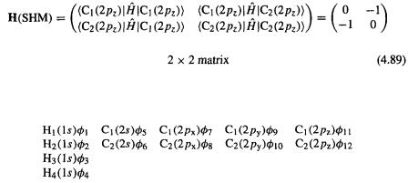
on  and the SHM Fock matrix is (using the compact Dirac notation
To write down the EHM Fock matrix, let us label the valence orbitals like this:

142 Computational Chemistry
Then
The SHM and EHM basis sets are shown in Fig. 4.26.
(2)The EHM Fock matrix interactions  do not have just two values
  or
or  as
as
in the SHM, but are functions of the orbitals (the basis functions)  and
and  and of the separation of these orbitals, as explained in (3) below.
(3)The EHM matrix elements  and
and  are calculated (rather than set equal to 0 or –1), although the calculation is a simple one using overlap integrals
and experimental ionization energies; in ab initio calculations (chapter 5) and more advanced SE calculations (chapter 6), the mathematical form of  taken into account. The
  -type interactions are taken as being proportional to the negative of the ionization
energy [55] of the orbital  and the
  -type interactions as being proportional to the overlap integral between
  and
and  and the negative of the average of the ionization
energies  and
and  of
of  and
and  (the negative of the orbital ionization energy is the energy of an electron in the orbital, compared to the zero of energy of the electron and the ionized species infinitely separated and at rest):
A proportionality constant K of about 2 is commonly used.
For
 and
and experiment shows

Introduction to Quantum Mechanics 143
The overlap integrals are calculated using Slater-type (section 5.3.2) functions for the basis functions, e.g.
where the parameters  depend on the particular atom (H, C, etc.) and orbital
  etc. The variable
  – R is the distance of the electron from the atomic nucleus on which the function is centered;
  is the vector from the origin of the Cartesian coordinate system to the electron, and R is the vector from the origin to the nucleus on which the basis function is centered:
where |
|
are the coordinates of the nucleus bearing the Slater function. The |
|
Slater function is thus a function of three variables |
and depends parametrically |
||
on the |
location |
of the nucleus A on which it is centered. The Fock matrix |
|
elements are thus calculated with the aid of overlap integrals whose values depend the location of the basis functions; this means that the MOs and their energies will depend on the actual geometry used in the input, whereas in a simple Hückel calculation, the MOs and their energies depend only on the connectivity of the molecule).
(4) The overlap matrix S in the EHM is not simply treated as a unit matrix, in effect ignoring it, for the purpose of diagonalizing the Fock matrix. Rather, the overlap integrals are actually evaluated, not only to help calculate the Fock elements, but also
to reduce the equation |
to the standard eigenvalue form |
This |
|
is done in the following way. Suppose the original set of basis functions |
could |
||
be transformed by some process into an orthonormal set |
(since atom-centered |
||
basis functions cannot be orthogonal, as explained in section 4.3.4, the new set must be delocalized over several centers and is in fact a linear combination of the atom-centered
set) such that with a new set of coefficients |
we have LC AO MOs with the same energy |
||||||
levels as before, i.e. |
|
|
|
|
|
|
|
where |
is the Kronecker delta (Eq. (4.57)). The result of the process referred to |
||||||
above is |
|
|
|
|
|
|
|
not |
as the energy will not depend on manipulation of a given set ofbasis functions) |
||||||
where the matrices H, C, S and |
were defined in section 4.3.4 (Eqs (4.55)) and |
and |
|||||
are analogous to H and S with |
in place of |
and |
is the matrix of coefficients |
||||
that satisfies the equation with the energy |
levels |
(the elements of |
being the same |
||||
as in the original equation |
Since from Eq. (4.97) |
the unit matrix |
|||||
(section 4.3.3), Eq. (4.98) simplifies to |
|
|
|
|
|
||
144 Computational Chemistry
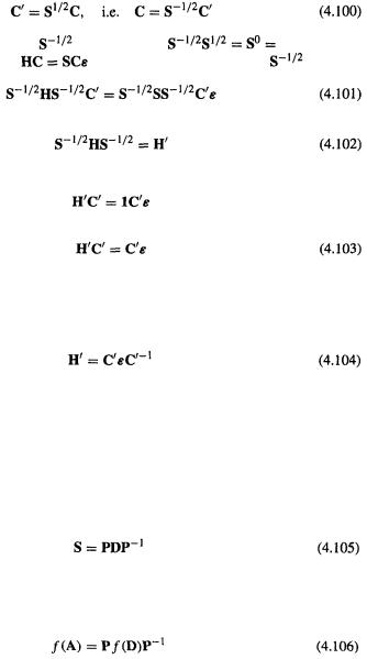
The Process that effects the transformation is called orthogonalization, since the result is to make the basis functions orthogonal. The favored orthogonalization procedure in computational chemistry, which I will now describe, is Löwdin orthogonalization (after the quantum chemist Per-Olov Löwdin).
Define a matrix  such that
(By multiplying on the left by |
and noting that |
1.) |
Substituting (4.100) into |
and multiplying on the left by |
we get |
Let
and note that  then we have from (4.101) and (4.102)
i.e.
Thus the orthogonalizing Process of (4.99) (or rather one possible orthogonalization process, Löwdin orthogonalization) is the use of an orthogonalizing matrix  to transform H by preand postmultiplication (Eq. 102) into
  satisfies the standard eigenvalue equation (Eq. (4.103)), so
In other words, using  we transform the original Fock matrix H, which is not directly diagonalizable to eigenvector and eigenvalue matrices C and
  into a related matrix
  which is diagonalizable to eigenvector and eigenvalue matrices
  and
and  The matrix
  is then transformed to the desired C by multiplying by
  (Eq. (4.100)). So without using the drastic
  approximation we can use matrix diagonalization to get the coefficients and energy levels from the Fock matrix.
The orthogonalizing matrix  is calculated from S: the integrals S are calculated and assembled into S, which is then diagonalized:
Now it can be shown that any function of a matrix A can be obtained by taking the same function of its corresponding diagonal alter ego and preand postmultiplying by the diagonalizing matrix P and its inverse 
and diagonal matrices have the nice property that  is the diagonal matrix whose diagonal element i, j = f (element i, j of D). So the inverse square root of D is the

Introduction to Quantum Mechanics 145
matrix whose elements are the inverse square roots of the corresponding elements of D. Therefore
and to find  we (or rather the computer) simply take the inverse square root of the diagonal (i.e. the nonzero) elements of D. To summarize: S is diagonalized to give
  and D, D is used to calculate
  then the orthogonalizing matrix
  is calculated (Eq. (4.107)) from
  and
and  The orthogonalizing matrix is then used to convert H to
  which can be diagonalized to give the eigenvalues and the eigenvectors (section 4.4.2).
Review of the EHM procedure
The EHM procedure for calculating eigenvectors and eigenvalues, i.e. coefficients (or in effect MOs – the  along with the basis functions comprise the MOs) and energy levels, bears several important resemblances to that used in more advanced methods (chapters 5 and 6) and so is worth reviewing.
(1) An input structure (a molecular geometry) must be specified and submitted to calculation. The geometry can be specified in Cartesian coordinates (probably the usual way nowadays) or as bond lengths, angles and dihedrals (internal coordinates), depending on the program. In practice a virtual molecule would likely be created with an interactive model-building program (usually by clicking together groups and atoms) which would then supply the EHM program with either Cartesian or internal coordinates.
(2)The EHM program calculates the overlap integrals S and assembles the overlap matrix S.
(3)The program calculates the Fock matrix elements  (Eqs (4.91)
and (4.92)) using stored values of ionization energies I, the overlap integrals S, and the proportionality constant K of that particular program. The matrix elements are assembled into the Fock matrix H.
(4)The overlap matrix is diagonalized to give P, D and  (Eq. (4.105)) and
  is then calculated by finding the inverse square roots of the diagonal elements of D. The orthogonalizing matrix
  is then calculated from P,
  and
and  (Eq. (4.107)).
(5)The Fock matrix H in the atom-centered nonorthogonal basis  is transformed into the matrix
  in the delocalized, linear combination orthogonal basis
  by preand postmultiplying H by the orthogonalizing matrix
  (Eq. (4.102)).
(6)  is diagonalized to give
  and
and  (Eq. (4.104)). We now have the energy levels
  (the diagonal elements of the
  matrix).
(7)  must be transformed to give the coefficients c of the original, atom-centered set of basis functions
  in the MOs (i.e. to convert the elements
  to
to  To get the
  in the
  we transform
  to C by premultiplying by
(Eq. (4.100)).
Molecular energy and geometry optimization in the EHM
Steps (1)–(7) take an input geometry and calculate its energy levels (the elements of 
and their MOs or wavefunctions (the |
from the c’s, the elements of C, and the basis |
|
functions |
Now, clearly any method in which the energy of a molecule depends on its |
|