


Molecular Mechanics 45
with their geometry, were formulated in 1946 by Westheimer1 and Meyer [3a], and by Hill [3b], In this same year Dostrovsky, Hughes2 and Ingold3 independently applied MM concepts of to the quantitative analysis of the reaction, but they do not seem to have recognized the potentially wide applicability of this approach [3c]. In 1947 Westheimer [3d] published detailed calculations in which MM was used to estimate the activation energy for the racemization of biphenyls.
Major contributors to the development of MM have been Schleyer4 [2b,c] and Allinger5 [1c,d]; one of Allinger’s publications on MM [1d] is, according to the Citation Index, one of the most frequently cited chemistry papers. The Allinger group has, since the 1960s, been responsible for the development of the “MM-series” of programs, commencing with MM1 and continuing with the currently widely-used MM2 and MM3, and the recent MM4 [4]. MM programs [5] like Sybyl and UFF will handle molecules involving much of the periodic table, albeit with some loss of accuracy that one might expect for trading breadth for depth, and MM is the most widely-used method for computing the geometries and energies of large biological molecules like proteins and nucleic acids (although recently SE (chapter 6) and even ab initio (chapter 5) methods have begun to be applied to these large molecules).
3.2THE BASIC PRINCIPLES OF MM
3.2.1 Developing a forcefield
The potential energy of a molecule can be written
where  etc. are energy contributions from bond stretching, angle bending, torsional motion (rotation) around single bonds, and interactions between atoms or groups which are nonbonded (not directly bonded together). The sums are over all the bonds, all the angles defined by three atoms A–B–C, all the dihedral angles defined by four atoms A–B–C–D, and all pairs of significant nonbonded interactions. The mathematical form of these terms and the parameters in them constitute a particular forcefield. We can make this clear by being more specific; let us consider each of these four terms.
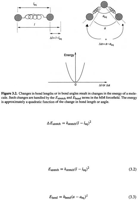
The bond stretching term. The increase in the energy of a spring (remember that we are modelling the molecule as a collection of balls held together by springs) when it is
1 Frank H. Westheimer, born Baltimore, Maryland, 1912. Ph.D. Harvard 1935. Professor University of Chicago, Harvard.
2 Edward D. Hughes, born Wales, 1906. Ph.D. University of Wales, D.Sc. University of London. Professor, London. Died 1963.
3Christopher K. Ingold, born London 1893. D.Sc. London 1921. Professor Leeds, London. Knighted 1958. Died London 1970.
4Paul von R. Schleyer, born Cleveland, Ohio, 1930. Ph.D. Harvard 1957. Professor Princeton; institute codirector and professor University of Erlangen-Nürnberg, 1976–1998. Professor University of Georgia.
5Norman L. Allinger, born Rochester New York, 1930. Ph.D. University of California at Los Angeles, 1954. Professor Wayne State University, University of Georgia.
46 Computational Chemistry
stretched (Fig. 3.2) is approximately proportional to the square of the extension:
where  is the proportionality constant (actually one-half the force constant of the spring or bond [6]; but note the warning about identifying MM force constants with the traditional force constant from, say, spectroscopy – see section 3.3); the bigger
  the stiffer the bond/spring – the more it resists being stretched; l is the length of the bond when stretched; and
 is the equilibrium length of the bond, its “natural” length.
If we take the energy corresponding to the equilibrium length  as the zero of energy, we can replace
  by
by 
The angle bending term. The increase in energy of system ball–spring–ball–spring– ball, corresponding to the triatomic unit A–B–C (the increase in “angle energy”) is approximately proportional to the square of the increase in the angle (Fig. 3.2); analogously to Eq. (3.2):
where  is a proportionality constant (one-half the angle bending force constant [6]; note the warning about identifying MM force constants with the traditional force constant from, say, spectroscopy –see section 3.3); a is the size of the angle when distorted; and
  is the equilibrium size of the angle, its “natural” value.
Molecular Mechanics 47
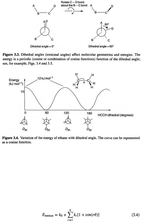
The torsional term. Consider four atoms sequentially bonded: A–B–C–D (Fig. 3.3). The dihedral angle or torsional angle of the system is the angle between the A–B bond and the C–D bond as viewed along the B–C bond. Conventionally this angle is considered positive if regarded as arising from clockwise rotation (starting with A–B covering or eclipsing C–D) of the back bond (C–D) with respect to the front bond (A–B). Thus in Fig. 3.3 the dihedral angle A–B–C–D is 60° (it could also be considered as being –300°). Since the geometry repeats itself every 360°, the energy varies with the dihedral angle in a sine or cosine pattern, as shown in Fig. 3.4 for the simple case of ethane. For systems A–B–C–D of lower symmetry, like butane (Fig. 3.5), the torsional potential energy curve is more complicated, but a combination of sine or cosine functions will reproduce the curve:

48 Computational Chemistry
The nonbonded interactions term. This represents the change in potential energy with distance apart of atoms A and B that are not directly bonded (as in A–B) and are not bonded to a common atom (as in A–X–B); these atoms, separated by at least two atoms (A–X–Y–B) or even in different molecules, are said to be nonbonded (with respect to each other). Note that the A–B case is accounted for by the bond stretching term  and the A–X–B term by the angle bending term
  but the nonbonded term
  is, for the A–X–Y–B case, superimposed upon the torsional term
  we can think of
  as representing some factor inherent to resistance to rotation about a (usually single) bond X–Y (MM does not attempt to explain the theoretical, electronic basis of this or any other effect), while for certain atoms attached to X and Y there may also be nonbonded interactions.
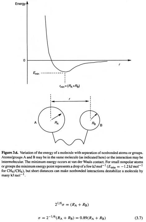
The potential energy curve for two nonpolar nonbonded atoms has the general form shown in Fig. 3.6. A simple way to approximate this is by the so-called Lennard–Jones 12-6 potential [7]:
where r is the distance between the centers of the nonbonded atoms or groups.
The function reproduces the small attractive dip in the curve (represented by the negative term) as the atoms or groups approach one another, then the very steep rise in potential energy (represented by the raising the positive, repulsive term raised to a large power) as they are pushed together closer than their van der Waals radii. Setting  we find that for the energy minimum in the curve the corresponding value of is i.e.
Molecular Mechanics 49
If we assume that this minimum corresponds to van der Waals contact of the nonbonded groups, then  the sum of the van der Waals radii of the groups A and B. So
and so
Thus  can be calculated from
  or estimated from the van der Waals radii.