

Ab initio calculations 231
calculations and the level at which one might need to work to obtain trustworthy results by [54].
Oxirene (oxacyclopropene) provides a canonical example of a molecule which even at the highest current levels of theory has declined to reveal its basic secret: can it exist (“Oxirene: to Be or Not to Be?” [44b]). Very large basis sets and advanced post-HF methods suggest it is a true minimum on the potential energy surface, but its disconcerting tendency to display an imaginary (section 2.5) calculated ring-opening vibrational mode at some of the highest levels used leaves the judicious chemist with no choice but to reserve judgement on its being. The nature of a series of substituted oxirenes, studied likewise at high levels, appears to be clearer [44a].
Another system that has yielded results which are dependent on the level of theory used, but which unlike the oxirene problem provides a textbook example of a smooth gradation in the nature of the answers obtained, is the ethyl cation (Fig. 5.17). At the HF STO-3G and 3-21G levels the classical structure is a minimum and the bridged nonclassical structure is a transition state, but with the 6-31G* basis the bridged ion has become a minimum and the classical one, although the global minimum, is not securely ensconced as such, being only  lower than the bridged ion. At the post-HF (section 5.4) MP2 level with the 6-31G* basis the bridged ion is a minimum and the classical one has lost the dignity of being even a stationary point. The ethyl cation and several other systems have been reviewed [54].
In summary, in many cases [32] the 3-21G (i.e.  or 6-31G* basis sets, or even the much faster molecular mechanics (chapter 3) or semiempirical (chapter 6) methods, are entirely satisfactory, but there are problems that require quite high levels of attack. In this connection, whether one chooses to regard the wide variety of basis sets at our disposal as representing a “chaotic proliferation” [55] or rather valuable components of our armamentarium is perhaps a matter of viewpoint.
5.4 POST-HF CALCULATIONS: ELECTRON CORRELATION
5.4.1 Electron correlation
Electron correlation is the phenomenon of the motion of pairs of electrons in atoms or molecules being connected (“correlated”) [56]. The purpose of post-HF calculations is to treat such correlated motion better than does the HF method. In the HF treatment, electron–electron repulsion is handled by having each electron move in a smeared-out, average electrostatic field due to all the other electrons (sections 5.2.3.2 and 5.2.3.6b), and the probability that an electron will have a particular set of spatial coordinates at some moment is independent of the coordinates of the other electrons at that moment. In reality, however, each electron at any moment moves under the influence of the repulsion, not of an average electron cloud, but rather of individual electrons (in fact current physics regards electrons as point particles – with wave properties of course). The consequence of this is that the motion of an electron in a real atom or molecule is more complicated than that for an electron moving in a smeared-out field [57] and the electrons are thus better able to avoid one another. Because of this enhanced (compared to the HF treatment) standoffishness, electron–electron repulsion is really smaller than

Ab initio calculations 233
spin coordinates would then be the same and the Slater determinant (section 5.2.3.1) representing the total molecular wavefunction would vanish, since a determinant is zero if two rows or columns are the same (section 4.3.3). This is just a consequence of the antisymmetry ofthe wavefunction: switching rows orcolumns ofa determinant changes its sign; for two rows/columns the same and
and  so
so  If the wavefunction were to vanish so would the electron density, which can be calculated from the wavefunction. This is one way of looking at the Pauli exclusion principle. Now, since the probability is zero that at any moment two electrons of like spin are at the same point in space, and since the wavefunction is continuous, the probability of finding them at a given separation should decrease smoothly with that separation. This means that even if electrons were uncharged, with no electrostatic repulsion between them, around each electron there would still be a region increasingly (the closer we approach the electron) unfriendly to other electrons of the same spin. This quantum mechanically engendered “Pauli exclusion zone” around an electron is called a Fermi hole (after Enrico Fermi; it applies to fermions (section 5.2.2) in general). It can be shown that the HF method overestimates the size ofthe Fermi hole. Besides the quantum mechanical Fermi hole, each electron in a real molecule, not in a “HF molecule”, is surrounded by a region unfriendly to all other electrons, regardless of spin, because of the electrostatic (Coulomb) repulsion between point particles (= electrons). This electrostatic exclusion zone is called a Coulomb hole. Since the HF method does not treat the electrons as discrete point particles it essentially ignores the existence of the Coulomb hole, allowing electrons to get too close on the average. This is the main source of the overestimation of electron–electron repulsion in the HF method. Post-HF calculations attempt to allow electrons, even of different spin, to avoid one another better than in the HF approximation.
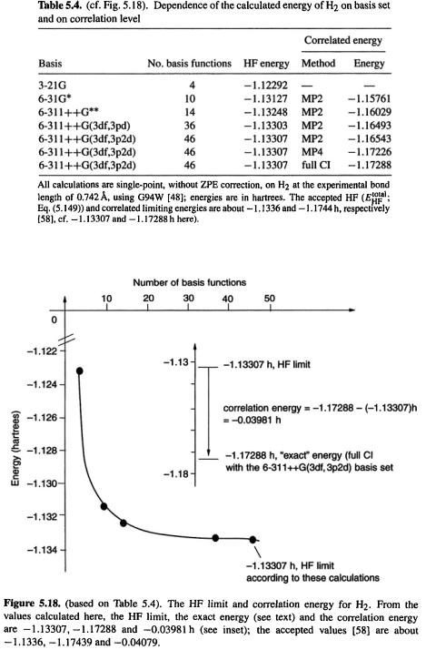
Hartree-Fock calculations give an electronic energy (and thus a total internal energy, section 5.2.3.6d) that is too high (the variation theorem, section 5.2.3.3, assures us that the HF energy will never be too low). This is partly because of the overestimation of electronic repulsion and partly because of the fact that in any real calculation the basis set is not perfect. For sensibly-developed basis sets, as the basis set size increases the HF energy gets smaller, i.e. more negative. The limiting energy that would be given by an infinitely large basis set is called the HF limit (i.e. the energy in the HF limit). Table 5.4 and Fig. 5.18 show the results of some HF and post-HF calculations on the hydrogen molecule; the limiting energies are close to the accepted ones [58]. Errors in energy, or in any other molecular feature, that can be ascribed to using a finite basis set are said to be caused by basis set truncation. Basis set truncation does not always cause serious errors; for example, the small HF/3-21G basis often gives good geometries (section 5.3.3). Where necessary, the truncation problem can be minimized by using a large (provided the size of the molecule makes this practical), appropriate basis set.
A measure of the extent to which any particular ab initio calculation does not deal perfectly with electron correlation is the correlation energy. In a canonical exposition [59] Löwdin defined correlation energy thus: “The correlation energy for a certain state with respect to a specified Hamiltonian is the difference between the exact eigenvalue of the Hamiltonian and its expectation value in the HF approximation for the state under consideration.” In other words, the correlation energy for a calculation on some molecule or atom is the energy calculated by some perfect quantum mechanical procedure,
234 Computational Chemistry
Ab initio calculations 235
minus the energy calculated by the HF method with a huge (“infinite”) basis set, using the same Hamiltonian:
 – E(HF limit) using the same Hamiltonian for both terms
From this definition the correlation energy is negative, since E(exact) is more negative than E(HF limit). Usually E(exact) and E(HF limit) are taken as the energy from a Hamiltonian that excludes relativistic effects (like that in section 5.2.2, Eqs (5.4), (5.5), (5.6) and associated discussion), which are significant only for heavy atoms, so unless qualified the term correlation energy means nonrelativistic correlation energy. The correlation energy is essentially the energy that the HF procedure fails to account for. If relativistic effects (and other , usually small, effects like spin–orbit coupling) are negligible then  is the difference between the experimental value (of the energy required to dissociate the molecule or atom into infinitely separated nuclei and electrons) and the limiting HF energy.
A distinction is sometimes made between dynamic and nondynamic or static correlation energy. Dynamic correlation energy is the energy a HF calculation does not account for because it fails to keep the electrons sufficiently far apart; this is the usual “correlation energy”. Nondynamic correlation energy is the energy a calculation (HF or otherwise) may not account for because it uses a single determinant, or starts from a single determinant (is based on a single-determinant reference – section 5.4.3); this problem arises with singlet diradicals, e.g. where a closed-shell description of the electronic structure is qualitatively wrong. Dynamic correlation energy can be calculated (“recovered”) by Møller-Plesset or configuration interaction methods (sections 5.4.2 and 5.4.3) and static correlation energy can be recovered by basing the wavefunction on more than one determinant, as in the multireference configuration interaction method (section 5.4.3).
Although HF calculations are satisfactory for many purposes (sections 5.5 and 5.6) there are cases where a better treatment of electron correlation is needed. This is particularly true for the calculation of relative energies, although geometries and some other properties are also improved by post-HF calculations, section 5.4). As an illustration of a shortcoming of HF calculations consider an attempt to find the C/C single bond dissociation energy of ethane by comparing the energy of ethane with that of two methyl radicals:
Let us simply subtract the energy of two methyl radicals from that of an ethane molecule, and compare with experiment the results of HF calculations and (anticipating section 5.4.2) the post-HF(i.e. correlated) MP2 method. In Table5.5 the energies shown for and
and  are the “uncorrected” ab initio energies (the energy displayed at the end ofany calculation; this is the electronic energy+the internuclear repulsion), the ZPE, and the “corrected” energy (uncorrected energy + ZPE); see section 5.2.3.6d. The ZPEs used here are from HF/6-31G* optimization/frequency jobs; these are fairly fast and give reasonable ZPEs. The ZPEs were all calculated by multiplying by an empirical correction factor of 0.9135 (this brings them into better agreement with experiment [60]). Although frequencies must be calculated with the same method (HF, MP2, etc.)

236 Computational Chemistry
and basis set as were used for the geometry optimization, ZPEs from a particular method/basis may be used to correct energies obtained with another method/basis. The only calculations that give reasonable agreement with the experimental ethane C–C dissociation energy (reported at from 368 to 377 kJ  [61]) are the correlated (MP2) ones, 370 and 363 kJ
  because of error in the experimental value the two MP2 results may be equally good. The HF values (248 and 232 kJ
  ) are very poor, even (especially!) when the very large 6-311++G(3df,3p2d) basis is used.
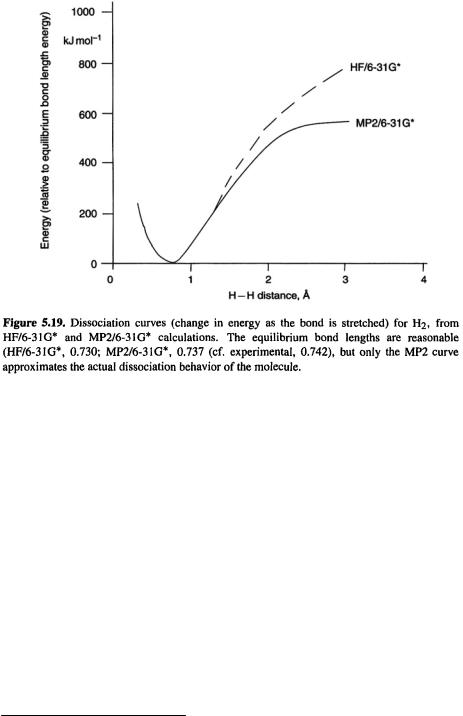
This inability of HF calculations to model correctly homolytic bond dissociation is commonly illustrated by curves of the change in energy as a bond is stretched, e.g. Fig. 5.19. The phenomenon is discussed in detail in numerous expositions of electron correlation [62]. Suffice it to say here that representing the wavefunction as one determinant (or a few), as is done in Hartree-Fock theory, does not permit correct homolytic dissociation to two radicals because while the reactant (e.g.  ) is a closedshell species that can (usually) be represented well by one determinant made up ofpaired electrons in the occupied MOs, the products are two radicals, each with an unpaired electron. Ways of obtaining satisfactory energies, with and without the use of electron correlation methods, for processes involving homolytic cleavage, are discussed further in section 5.5.2.

 where
where  is the sum of one-electron energies and internuclear repulsions and
  is the
  , the molecule for which a HF (i.e. an SCF) calculation was shown in detail in section 5.2.3.6e. As for the HF calculation, we will take the internuclear distance as 0.800 Å and use the STO-1G basis set; we can then use for our MP2 calculation these HF results that we obtained in section 5.2.3.6e:
 (recall that these are respectively the coefficient of basis function 1,
  in MO1 and the coefficient of basis function 2,
  in MO1. In this simple case there is one function on each atom:
  and
and  on atoms
 The two-electron repulsion integrals:
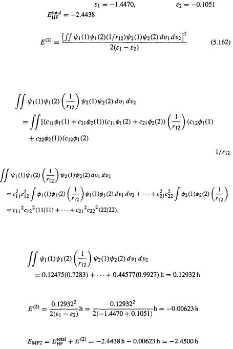
|
Ab initio calculations 239 |
The energy levels: occupied MO, |
virtual MO, |
The HF energy: |
|
The MP2 energy correction for a closed-shell two-electron/two-MO system is [70]:
Applying this formula is straightforward; although the arithmetic is tedious, it is worth doing (as was true for the HF calculation in section 5.2.3.6e) in order to appreciate how much work is involved in even this simplest molecular MP2 job. Consider the integral in the numerator of Eq. (5.162); substituting for  and
and 
Multiplying out the integrand gives a total of 16 terms (from 4 terms to the left of and 4 terms to the right), and leads to a sum of 16 integrals:
recalling the notational degeneracy in the two-electron integrals (section 5.2.3.6e, “Step 2 Calculating the integrals”). Substituting the values of the coefficients and the two-electron integrals:
So from Eq. (5.162)
The MP2 energy is the HF energy plus the MP2 correction (Eq. (5.162)):
This energy, which includes internuclear repulsion, since  includes this (Eq. (5.93)), is the MP2 energy normally printed out at the end of the calculation. To get an intuitive feel for the physical significance of the calculation just performed look again at Eq. (5.162), which applies to any two-electron/two-basis function species.
240 Computational Chemistry
The equation shows that the absolute value (the correction is negative since is smaller than
  – the occupied MO has a lower energy than the virtual one) of the correlation correction increases, i.e. the energy decreases, with the magnitude of the integral (which is positive). This integral represents the decrease in energy arising from allowing an electron pair in the occupied MO
  to spill over into the virtual MO
represents electron 1 in |
and |
represents electron 2 in |
|
|
represents electron 1 in |
and |
represents electron 2 in |
|
|
The operator |
brings in coulombic interaction: the coulombic repulsion energy |
|||
between infinitesimal volume elements |
|
and |
separated |
|
by a distance |
is |
|
and the integral is simply |
|
the sum over all such volume elements (cf. the discussion in connection with Fig. 5.3 and the average-field integrals J and K in section 5.2.3.2). Physically, the decrease in energy makes sense: allowing the electrons to be partly in the formally unoccupied virtual MO rather than confining them strictly to the formally occupied MO enables them to avoid one another better than in the HF treatment, which is based on a Slater determinant consisting only of occupied MOs (section 5.2.3.1). The essence of the MP method (MP2, MP3, etc.) is that the correction term handles electron correlation by promoting electrons from occupied to unoccupied (virtual) MOs, giving electrons, in some sense, more room to move and thus making it easier for them to avoid one another; the decreased interelectronic repulsion results in a lower electronic energy. The
contribution of the |
interaction” to |
decreases as the occupied/virtual MO |
|
gap |
increases, since this is in the denominator. Physically, this makes sense: the |
||
bigger the gap between the occupied and higher-energy virtual MO, the “harder” it is to promote electrons from the one into the other, so the less can such promotion contribute to electronic stabilization. So in the expression for  (Eq. (5.162), the numerator represents the promotion of electrons from the occupied to the virtual orbital, and the denominator represents how hard it is to do this.
As we just saw, MP2 calculations utilize the HF MOs (their coefficients c and energies  ). The HF method gives the best occupied MOs obtainable from a given basis set and a one-determinant total wavefunction
  but it does not optimize the virtual orbitals (after all, in the HF procedure we start with a determinant consisting of only the occupied MOs – sections 5.2.3.1–5.2.3.4). To get a reasonable description of the virtual orbitals and to obtain a reasonable number of them into which to promote electrons, we need a basis set that is not too small. The use of the STO-1G basis in the above example was purely illustrative; the smallest basis set generally considered acceptable for MP calculations is the 6-31G*, and in fact this is perhaps the one most frequently used for MP2 calculations. The 6-311G** basis set is also widely used for MP2 and MP4 calculations. Both bases can of course be augmented (section 5.3.3) with diffuse functions, and the 6-31G* with H polarization functions (6-31G**). MP2 calculations
increase rapidly in complexity with the number of electrons |
and orbitals, involving |
as they do a sum of terms (rather than just one term as in |
), each representing |
the promotion of an electron pair from an occupied to a virtual orbital; thus an MP2 calculation on  with the 6-31G* basis involves 8 electrons and 19 MOs (4 occupied and 15 virtual MOs).
Ab initio calculations 241
In MP2 calculations doubly excited states (doubly excited configurations) interact with the ground state (the integral in Eq. (5.162) involves  with electrons 1 and 2, and
  with electrons 1 and 2). In MP3 calculations doubly excited states interact with one another (there are integrals involving two virtual orbitals). In MP4 calculations singly, doubly triply and quadruply excited states are involved. MP5 and higher expressions have been developed, but MP2 and MP4 are by far the most popular MP levels (also called MBPT(2) and MBPT(4) – many-body perturbation theory). MP2 calculations, which are much slower than HF, can be speeded up somewhat by specifying MP2(FC),
MP2 frozen-core, in contrast to MP2(FULL); frozen-core means that the core (nonvalence electrons) are “frozen,” i.e. not promoted into virtual orbitals, in contrast to full MP2 which takes all the electrons into account in summing the contributions of excited states to the lowering of energy. Most programs (e.g. Gaussian, Spartan) perform MP2(FC) by default when MP2 is specified, and “MP2” usually means frozen-core. MP4 calculations are sometimes done omitting the triply excited terms (MP4SDQ) but the most accurate (and slowest) implementation is MP4SDTQ (singles, doubles, triples, quadruples).
Calculated properties like geometries and relative energies tend to be better (to be closer to the true ones) when done with correlated methods (sections 5.5.1–5.5.4). To save time, energies are often calculated with a correlated method on a HF geometry, rather than carrying out the geometry optimization at the correlated level. This is called a single-point calculation (it is performed at a single point on the HF potential energy surface, without changing the geometry). A single-point MP2(FC) calculation using the 6-311G** basis, on a structure that was optimized with the HF method and the 6-31G* basis, is designated as MP2(FC)/6-311G**//HF/6-31G*. A HF/6-31G* (say) geometry optimization, without a subsequent single-point calculation, is sometimes designated HF/6-31G*//HF/6-31G*, and an MP2 optimization MP2/6-31G*//MP2/6-31G*. The correlation treatment (HF, MP2, MP4,...) is often called the method, and the basis set (STO-3G, 3-21G, 6-31G*,...) the level, but we will often find it convenient to let level denote the combined procedure of method and basis set, referring, say, to an MP2/6-31G* calculation as being at a higher level than an HF/6-31* one.
Figure 5.20 shows the rationale behind the use of single-point calculations for obtaining relative energies. In the diagram a single-point MP2 calculation on a stationary point at the HF geometry gives the same energy as would be obtained by optimizing the species at the MP2 level, which is often approximately true (it would be exactly true if the MP2 and HF geometries were identical). For example, the single-point and optimized energies of butanone are –231.68593 and –231.68818h, a difference of 0.00225 h (2.3 mh) or not large bearing in mind that special high-accuracy calculations (section 5.5.2.2) are needed to reliably get relative energies to within, say,
  Single-point calculations would also give relative energies similar to those from the use of optimized correlated geometries if the incremental deviations from the optimized-geometry energies were about the same for the two species being compared (e.g. reactant and TS for an activation energy, reactant and product for a reaction energy).
The method can occasionally give not just quantitatively, but qualitatively wrong results. The HF and correlated surfaces may have different curvatures: for example a minimum on one surface may be a transition state or may not exist (may not be a stationary point) on another. Thus fluoroand difluorodiazomethane are HF minima but