Density Functional Calculations 399
a system of noninteracting electrons with electron density equal to the real system (of course the basis set used imposes a limit on the accuracy of the molecular orbitals and thus on 
Including in an LSDA gradient-corrected DFT expression for
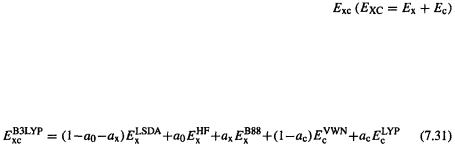
a weighted contribution of the expression for  gives a HF/DFT exchange-correlation functional, commonly called a hybrid DFT functional. The most popular hybrid functional at present (and in fact the most popular DFT functional) is based on an exchange-energy functional developed by Becke in 1993, and modified by Stevens et al. in 1994 by introduction of the LYP 1988 correlation-energy functional. This exchange-correlation functional, called the Becke3LYP or B3LYP functional [49] is
Here  is the kind of accurate “pure DFT” LSDA non-gradient-corrected exchange functional alluded to in section 7.2.3.4b,
  is the KS-orbital-based HF exchange energy functional of Eq. (7.30),
  is the Becke 88 exchange functional mentioned above,
  is the Vosko, Wilk, Nusair function (VWN, or Slater VWN, SVWN function), which forms part of the accurate functional for the homogeneous electron gas of the LDA and the LSDA (sections 7.2.3.4a and 7.2.3.4b), and
  is the LYP correlation functional mentioned above;
  and
and  of the last three terms are gradientcorrected. The parameters
 and
and are those that give the best fit of the calculated energy to molecular atomization energies. This is thus a gradient-corrected, hybrid functional. Of those functionals that have been around long enough to be well-tested, the B3LYP functional is, by and large, the most useful one (see the various applications of DFT, below). No doubt improved functionals will be discovered, and high hopes have been expressed for hybrid functionals by some of the chief pioneers in density functional theory: “A true marriage of density functional and Hartree-Fock ideas and technologies has emerged, and a potentially very beneficial cross-fertilization between DFT and traditional wave function methods has begun.” [13].
DFT calculations with functionals incorporating gradient corrections, or gradient corrections and the HF exchange term (hybrid functionals), can be speeded up with only a little loss in accuracy by a so-called perturbation method [50]. Here the KS equations ((7.23), (7.25)) are solved using the derivative  (Eq. (7.24)) corresponding to the LSDA functional, which is of course simpler than the gradient-corrected or hybrid functional. The energy is then calculated from Eq. (7.21), now using the gradient-corrected or hybrid functional. This is a perturbation approach because the “real” system with the better functional is regarded as a perturbation of the system with the approximate KS orbitals and corresponding electron density function. This perturbation method is available in some versions of Spartan [47] (see the discussion of gradient-corrected functionals, above) as a pBP/DN* or pBP/DN** calculation.
7.3 APPLICATIONS OF DENSITY FUNCTIONAL THEORY
Levine has compared geometries, energies, etc. from DFT with those from molecular mechanics, ab initio, and semiempirical methods [51]. Hehre [52] and Hehre and
400 Computational Chemistry
Lou [48] have provided extensive, very useful compilations of ab initio, semiempirical, DFT, and some molecular mechanics results. Calculations in this chapter by the author were done with the programs Titan [53] (B3LYP), Spartan [47] (pBP and MP2), Gaussian 94 [54], and Gaussian 98 [45] (for BP86, high-accuracy energies, and IR, UV, and NMR spectra).
7.3.1 Geometries
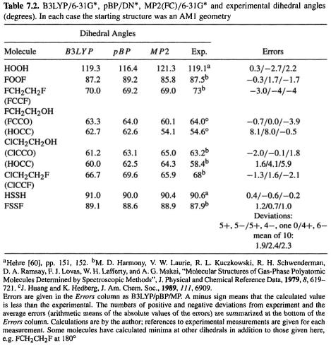
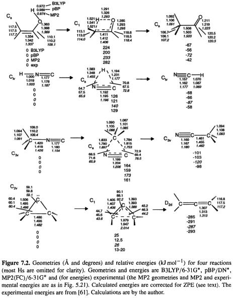
Building on the general considerations about the calculation of molecular geometries in section 5.5.1, we can examine the results of DFT geometry optimizations of the same set of 20 molecules that were used in Fig. 5.23, and Fig. 6.2. The geometries in Fig. 7.1 are analyzed in Table 7.1, and Table 7.2 gives the dihedral angles for the same eight molecules as in Table 5.8, and Table 6.2 (Fig. 7.1 corresponds to Figs 5.23 and 6.2, Table 7.1 to Tables 5.7 and 6.1, and Table 7.2 to Tables 5.8 and 6.2). The DFT methods chosen were B3LYP/6-31G* and pBP/DN*, which were mentioned in section 7.2.3.4c. The gradient-corrected hybrid B3LYP functional with the 6-31G* basis set was chosen because this is at present the most popular DFT method, and is available in most commercial computational chemistry packages that include DFT. The perturbationally implemented BP86 (section 7.2.3.4c) functional with the DN* numerical basis represents a gradient-corrected, non-hybrid method. It is found in some versions of Spartan, and was chosen because it is fast (see below) and comparable in accuracy to B3LYP/6-31G*. As mentioned above, it should give similar results to B88P86/6-311G* (designated BP86/6-311G* in Gaussian 98) calculations; in section 7.3.2.2b we will see that pBP/DN*, B88P86/6-31G*, and B88P86/6-311G* actually do seem to give very similar results. Here, we compare geometries from B3LYP/6-31G*, pBP/DN*, MP2(FC)/6-31G* (the highest-level ab initio method in routine use), and experiment.
This survey suggests that B3LYP/6-31G* gives excellent geometries, quite similar to those from MP2/6-31G*, and pBP/DN* gives good geometries. Only for bonds from C to O, N, F, Cl, or S is B3LYP/6-31 G* significantly worse than MP2, and about the same as pBP/DN*; apart from these, B3LYP/6-31G* bond lengths are mostly within 0.009 of experiment. pBP bond lengths are mostly within 0.026 of experiment. O–H bonds were always slightly too long by all three methods, and C–H bonds were always slightly too long for pBP/DN*. All three methods give bond angles usually within 1° of experiment
|
|
|
(the worst error was in the HCN angle of |
2.2° for pBP/DN*). The dihedral |
angles by all three methods are all mostly within .l°–3° of experiment, but |
and |
show somewhat larger errors (up to ca. 6°). The |
worst dihedral errors were ca. 8° for FCH2CH2F by the DFT methods, which is similar to the MP2/6-31G* error of 5.9° for the HOCC dihedral of 
The mean error in 39 (13 + 8 + 9 + 9) bond lengths is ca. 0.004–0.01 Å for B3LYP and MP2, and ca. 0.01–0.025 for pBP. The mean error in 18 bond angles is ca. 0.6° for the three methods. For the 10 dihedrals the mean error is ca. 2°.
Geometry errors for 108 molecules were reported by Scheiner et al. [55], comparing several ab initio and DFT methods. They found that Becke’s original three-parameter function (which they denote ACM, for adiabatic connection method; B3LYP was developed as a modification of this [49]), with a 6-31G*-type and with the 6-31G**
Density Functional Calculations 401
basis sets, gave average bond length errors of about 0.01 Å and bond angle errors of about 1.0°. They concluded that of the methods they examined ACM is the best choice for both geometries and reaction energies. St.-Amant et al. [56] also compared ab initio and DFT methods and found average dihedral angle errors of ca. 3° for 11 molecules using a perturbative gradient-corrected DFT method with an approximately
402 Computational Chemistry
Density Functional Calculations 403
404 Computational Chemistry
6-311G*-type basis set. These workers found average bond length errors of, e.g. 0.01 Å for C–H and 0.009 Å for C-C single bonds, and average bond angle errors of 0.5°. El-Azhary reported B3LYP with the 6-31G** and cc-pVDZ basis sets to give slightly better geometries than MP2, although MP2 avoids the occasional large errors given by B3LYP [57]. The effect of using different basis sets was minor. In a comparison of HF, MP2 and DFT (five functionals), Bauschlicher found B3LYP to be the best method overall [58].
B3LYP/6-31G*, pBP/DN*, and MP2(FC)/6-31G* geometries are further compared, for the species in four reaction profiles, in Fig. 7.2. These correspond to the ab initio comparisons of Fig. 5.21 and the semiempirical comparisons of Fig. 6.3. For the reactants and products, the DFT deviations from the MP2 geometries are not more than 0.026 Å  1.180Å cf. 1.154 Å) and 0.8°
 110.2° 110.2° cf. 109.4°). For the transition states the maximum deviations from the MP results are –0.107 Å
Density Functional Calculations 405
(HNC reaction, 1.383 Å cf. 1.455 Å) and –11.2° (HNC reaction, 54.7° cf. 65.9°). We can assume that the deviations here from the true geometries are similar for the reactants and products to the cases of other normal molecules, as discussed above, i.e. that the DFT results are good to excellent (with B3LYP probably better than pBP). For transition states experimental geometries are not yet available, and we cannot be sure that the MP2 geometries are superior to the DFT ones. The B3LYP and pBP geometries are quite similar, with the largest discrepancies again being in the transition state for