146 Computational Chemistry

geometry can in principle be used to find minima and transition states (see chapter 2). This brings us to the matter of how the EHM calculates the energy of a molecule. The energy of a molecule, that is, the energy of a particular nuclear configuration on the potential energy surface, is the sum of the electronic energies and the internuclear repulsions

In comparing the energies of isomers, or of two geometries of the same molecule, one should, strictly, compare The electronic energy is the sum of kinetic energy and potential energy (electron–electron repulsion and electron–nucleus attraction) terms. The internuclear repulsion, due to all pairs of interacting nuclei and trivial to calculate, is usually represented by V, a symbol for potential energy. The EHM ignores Furthermore, the method calculates electronic energy simply as the sum of one-electron energies (section 4.3.5), ignoring electron-electron repulsion. Hoffmann’s tentative justification [53a] for ignoring internuclear repulsion and using a simple sum of one-electron energies was that when the relative energies of isomers are calculated, by subtracting two values of the electron repulsion and nuclear repulsion terms approximately cancel, i.e. that changes in energy that accompany changes in geometry are due mainly to alterations of the MO energy levels. Actually, it seems that the (quite limited) success of the EHM in predicting molecular geometry is due to the fact that

is approximately proportional to the sum of the occupied MO energies; thus although the EHM energy difference is not equal to the difference in total energies, it is (or tends to be) approximately proportional to this difference [56]. In any case, the real strength of the EHM lies in the ability of this fast and widely applicable method to assist chemical intuition, if provided with a reasonable molecular geometry.

4.4.2An illustration of the EHM: the protonated helium molecule

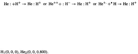
Protonation of a helium atom gives the helium hydride cation, the simplest heteronuclear molecule [57]. Conceptually, of course, this can also be formed by the union of a helium dication and a hydride ion, or a helium cation and a hydrogen atom:

Its lower symmetry makes this molecule better than for illustrating molecular quantum mechanical calculations (most molecules have little or no symmetry). Following the prescription in points (1)–(7), we calculate the following results.

(1) Input structure

We choose a plausible bond length: 0.800 Å (the H–H bond length is 0.742 Å and the H–X bond length is ca. 1.0 Å, where X is a “first-row” element (in quantum chemistry, first-row means Li to F, not H and He). The Cartesian coordinates could be written

(2) Overlap integrals and overlap matrix

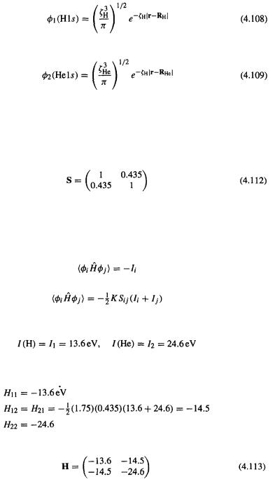
The minimal valence basis set here consists of the hydrogen 1s orbital and the helium 1s orbital The needed integrals are and where

148Computational Chemistry

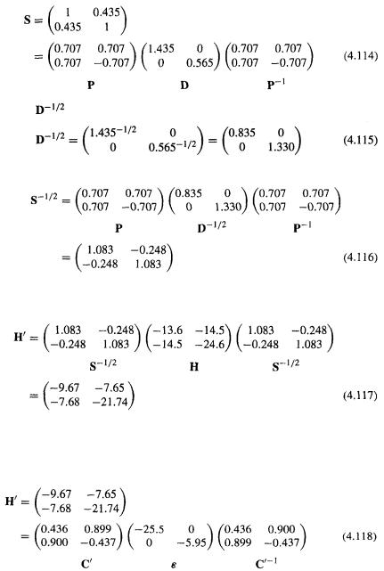
(4)Orthogonalizing matrix

As explained above, we (a) diagonalize S, (b) calculate then (c) calculate the orthogonalizing matrix

(a) Diagonalize S

(b)Calculate

(c)Calculate the orthogonalizing matrix

(5) Transformation of the original Fock matrix H to

Using Eq. (102):

(6) Diagonalization of

From Eq. (4.104) diagonalization of gives an eigenvector matrix and the eigenvalue matrix the columns of are the coefficients of the transformed,

orthonormal basis functions:

Introduction to Quantum Mechanics 149

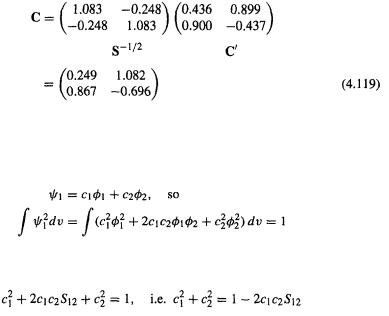
We now have the energy levels (–25.5 and –5.95 eV), but the eigenvectors of must be transformed to give us the coefficients of the original, nonorthogonal basis functions.

(7) Transformation of to C

Using Eq. (4.102),

Note that unlike the case in the SHM, the sum of the squares of the c’s for an MO does not equal 1, since overlap integrals for basis functions on different atoms are not set equal to 0; in other words, the basis functions are not assumed to be orthogonal, and the overlap matrix is not a unit matrix. Thus for

since the probability of finding an electron in somewhere in space is 1. The basis functions are normalized, so

4.4.3 The extended Hückel method – applications

The EHM was initially applied to the geometries (including conformations) and relative energies of hydrocarbons [53a], but the calculation of these two basic chemical parameters is now much better handled by SE methods like AM1 and PM3 (chapter 6) and by ab initio (chapter 5) methods. The main use of the EHM nowadays is to study large, extended systems [59] like polymers, solids and surfaces. Indeed, of four papers by Hoffmann and coworkers in the J. Am. Chem. Soc. in 1995, using the EHM, three applied it to such polymeric systems [60]. The ability of the method to illuminate problems in solid-state science makes it useful to physicists. Even when not applied to polymeric systems, the EHM is frequently used to study large, heavy-metal-containing molecules [61] that might not be very amenable to ab initio or to other SE approaches.

4.4.4 Strengths and weaknesses of the EHM

Strengths

One big advantage of the EHM over ab initio methods (chapter 5), more elaborate SE methods (chapter 6), and DFT methods (chapter 7), is that the EHM can be applied to

150 Computational Chemistry

very large systems, and can treat almost any element since the only element-specific parameter needed is an ionization energy, which is usually available. In contrast, more elaborate SE methods have not been parameterized for most elements (although recent parameterizations of PM3 and MNDO for transition metals make these much more generally useful than hitherto – chapter 6, section 6.2.6.7). For ab initio and DFT methods, basis sets may not be available for elements of interest, and besides, ab initio and even DFT methods are hundreds of times slower than the EHM and thus limited to much smaller systems. The applicability of the EHM to large systems and a wide variety of elements is one reason why it has been extensively applied to polymeric and solid-state structures. The EHM is faster than more elaborate SE methods because calculation of the Fock matrix elements is so simple and because this matrix needs to be diagonalized only once to yield the eigenvalues and eigenvectors; in contrast, SE methods like AM1 and PM3 (chapter 6), as well as ab initio calculations, require repeated matrix diagonalization because the Fock matrix must be iteratively refined in the SCF procedure (section 5.2.3.6).

The spartan reliance of the EHM on empirical parameters helps to make it relatively easy (in the right hands) to interpret its results, which depend, in the last analysis, only on geometry (which affects overlap integrals) and ionization energies. With a strong dose of chemical intuition this has enabled the method to yield powerful insights, such as counterintuitive orbital mixing [62], and the very powerful Woodward–Hoffmann rules [38].

The applicability to large systems, including polymers and solids, containing almost any kind of atom, and the relative transparency of the physical basis of the results, are the main advantages of the EHM.

Surprisingly for such a conceptually simple method, the EHM has a theoreticallybased advantage over otherwise more elaborate SE methods like AM1 and PM3, in that it treats orbital overlap properly: those other methods use the “neglect of differential overlap” or NDO approximation (section 6.2), meaning that they take as in the SHM. This can lead to superior results from the EHM [63].

The EHM is a very valuable teaching tool because it follows straightforwardly from the SHM yet uses overlap integrals and matrix orthogonalization in the same fashion as the mathematically more elaborate ab initio method.

Finally, the EHM, albeit more elaborately parameterized than in its original incarnation, has recently been shown to offer some promise as a serious competitor to the very useful and popular SE AM1 method (section 6.2.6.4) for calculating molecular geometries [64].

Weaknesses

The weaknesses of the standard EHM probably arise at least in part from the fact that it does not (contrast the ab initio method, chapter 5) take into account electron spin or electron–electron repulsion, ignores the fact that molecular geometry is partly determined by internuclear repulsion, and makes no attempt to overcome these defects by parameterization (unlike the recent variation which, with the aid of careful parameterization, evidently gives good geometries [64]).

The standard EHM gives, by and large, poor geometries and energies. Although it predicts a C–H bond length of ca. 1.0 Å, it yields C/C bond lengths of 1.92, 1.47 and