


 using single-point MP2/6-31 G* energies on HF geometries, is misguided if
  does not exist on the MP2 PES. Nevertheless, because HF optimizations followed by single-point correlated energy calculations are much faster (“cheaper”) than correlated optimizations, and usually give improved relative energies, the method is widely used. Figure 5.21 compares some MP2 singlepoint and MP2-optimized energies with experiment or with high-level calculations [72]. Geometries are discussed further in section 5.5.1.
Ab initio calculations 243

244 Computational Chemistry
adding on to the HF wavefunction terms that represent promotion of electrons from occupied to virtual MOs. The HF term and the additional terms each represent a particular electronic configuration, and the actual wavefunction and electronic structure of the system can be conceptualized as the result of the interaction of these configurations. This electron promotion, which makes it easier for electrons to avoid one another, is as we saw (section 5.4.2) also the physical idea behind the MP method; the MP and CI methods differ in their mathematical approaches.
HF theory (sections 5.2.3.1–5.2.3.6) starts with a total wavefunction or total MO  which is a Slater determinant made of “component” wavefunctions or
  In section 5.2.3.1 we approached HF theory by considering the Slater determinant for a
four-electron system:
To construct the HF determinant we used only occupied MOs: four electrons require only two spatial “component” MOs,  and
and  and for each of these there are two spin orbitals, created bymultiplying
  by one of the spin functions
  or
or  the resulting four spin orbitals
  are used four times, once with each electron. The determinant
  the HF wavefunction, thus consists of the four lowest-energy spin orbitals; it is the simplest representation of the total wavefunction that is antisymmetric and satisfies the Pauli exclusion principle (section 5.2.2), but as we shall see it is not a complete representation of the total wavefunction.
In the Roothaan–Hall implementation of ab initio theory each “component”  is composed of a set of basis functions (Sections 5.2.3.6 and 5.3):
Now note that there is no definite limit to how many basis functions  can be used for our four-electron calculation; although only two spatial
  and
and  (i.e. four spin orbitals) are required to accommodate the four electrons of this
  the total number of
  can be greater. Thus for the hypothetical H–H–H–H an STO-3G basis gives four
  a 3-21G basis gives 8, and a 6-31G** basis gives 20 (section 5.3.3). The idea behind CI is that a better total wavefunction, and from this a better energy, results if the electrons are confined not just to the four spin orbitals
 but are allowed to roam over all, or at least some, of the virtual spin orbitals
  To permit this we could write
  as a linear combination of determinants

Ab initio calculations 245
where  is the HF determinant of Eq. (5.163) and
  etc. correspond to the promotion of electrons into virtual orbitals, e.g. we might have
 was obtained from
  by promoting an electron from spin orbital
  to the spin orbital
  Another possibility is
Here two electrons have been promoted, from the spin orbitals  and
and  to
to  and
and  and
and  represent promotion into virtual orbitals of one and two electrons, respectively, starting with the HF electronic configuration (Fig. 5.22).

246 Computational Chemistry
Equation (5.165) is analogous to Eq. (5.164): in (5.164) “component” MOs  are expanded in terms of basis functions
  and in (5.165) a total MO
  is expanded in terms of determinants, each of which represents a particular electronic configuration. We know that the
  basis functions of Eq. (5.164) generate
  component MOs
  (section 5.2.3.6a), so the
  determinants of Eq. (5.165) must generate
  total wavefunctions
  and Eq. (5.165) should really be written
i.e. (cf. Eq. (5.164))
What is the physical meaning of all these totalwavefunctions  Each determinant D, or a linear combination of a few determinants, represents an idealized (in the sense of contributing to the real electron distribution) configuration, called a configuration state function or configuration function, CSF (see below). The CI wavefunctions of Eqs (5.168) or Eqs (5.169), then, are linear combinations of CSF’s. No single CSF fully represents any particular electronic state. Each wavefunction
 is the total wavefunction of one of the possible electronic states of the molecule, and the weighting factors
  in its expansion determine to what extent particular CSF’s (idealized electronic states)
contribute to any |
For the lowest-energy wavefunction |
representing the ground |
||
electronic state, we expect the HF determinant |
to make the largest contribution to the |
|||
wavefunction. Thewavefunctions |
etc. |
represent excited electronic states. The |
||
single-determinant HF wavefunction of Eq. (5.163) (or the general single-determinant
wavefunction of Eq. (5.12)) is merely an approximation to the |
of Eqs (5.168). |
If every possible idealized electronic state of the system, i.e. |
every possible deter- |
minant D, were included in the expansions of Eqs (5.168), then the wavefunctions  would be full CI wavefunctions. Full CI calculations are possible only for very small molecules, because the promotion of electrons into virtual orbitals can generate a huge number of states unless we have only a few electrons and orbitals. Consider for example a full CI calculation on a very small system, H–H–H–H with the 6-31G* basis set. We have eight basis functions and four electrons, giving eight spatial MOs and 16 spin
MOs, of which the lowest four are occupied. There are two |
electrons to be promoted |
into 6 virtual α spin MOs, i.e. to be distributed among 8 |
spin MOs, and likewise |
for the  electrons and
  spin orbitals. This can be done in
  ways. The number of configuration state functions is about half this number of determinants; a CSF is a linear combination of determinants for equivalent states, states which differ only by whether an
  or a
or a  electron was promoted. CI calculations with more than five billion (sic) CSFs have been performed on ethyne,
  rightly

Ab initio calculations 247
called benchmark calculations, such computational tours de force are, although of limited direct application, important for evaluating the efficacy, by comparison, of other methods.
The simplest implementation of CI is analogous to the Roothaan–Hall implementation of the HF method: Eqs (5.168) lead to a CI matrix, as the HF equations (using Eqs (5.164)) lead to a HF matrix (Fock matrix; section 5.2.3.6). We saw that the Fock
matrix F can be calculated from the |
and |
of Eq. (5.164) (starting with a “guess” |
||||
of the |
and that F (after transformation to an orthogonalized matrix |
and diag- |
||||
onalization) gives eigenvalues and eigenvectors |
i.e. F leads to the energy levels |
|||||
and thewavefunctions |
of the component MOs |
all this was shown in detail in |
||||
section 5.2.3.6e. Similarly, a CI matrix can be calculated in which the determinants D play the role that the basis functions  play in the Fock matrix, since the D’s in
Eqs (5.168) correspond mathematically to the |
in Eq. (5.164)). The D’s are com- |
||
posed of spin orbitals |
and |
and the spin factors can be integrated out, reducing |
|
the elements of the CI matrix to expressions involving the basis functions and coefficients of the spatial component MOs  The CI matrix can thus be calculated from the MOs resulting from an HF calculation. Orthogonalization and diagonalization of
the CI matrix gives the energies and the wavefunctions of the ground state |
and, |
|
from determinants, |
excited states. A full CI matrix would give the energies and |
|
wavefunctions of the ground state and all the excited states obtainable from the basis set being used. Full CI with an infinitely large basis set would give the exact energies of all the electronic states; more realistically, full CI with a large basis set gives good energies for the ground and many excited states.
Full CI is out of the question for any but small molecules, and the expansion of Eq. (5.169) must usually be limited by including only the most important terms. Which terms can be neglected depends partly on the purpose of the calculation. For example, in calculating the ground state energy quadruply excited states are, unexpectedly, much more important than triply and singly excited ones, but the latter are usually included too because they affect the electron distribution of the ground state, and in calculating excited state energies single excitations are important. A CI calculation in which all the post HF D’s involve only single excitations is called CIS (CI singles); such a calculation yields the energies and wavefunctions of excited states and often gives a reasonable account of electronic spectra. Another common kind of CI calculation is CI singles and doubles (CISD, which actually indirectly includes triply and quadruply excited states). Various mathematical devices have been developed to make CI calculations recover a good deal of the correlation energy despite the necessity of (judicious) truncation of the CI expansion. Perhaps the currently most widely-used implementations of CI are multiconfigurational SCF (MCSCF) and its variant complete active space SCF
(CASSCF), and the coupled-cluster (CC) and related quadratic CI (QCI) methods. The CI strict analogue of the iterative refinement of the coefficients that we saw
in HF calculations (section 5.2.3.6e) would refine just the weighting factors of the
determinants (the c’s of Eqs (5.168), but in the MCSCF version |
of CI the spatial |
MOs within the determinants are also optimized (by optimizing the |
of the LCAO |
expansion, Eq. (5.164)). A widely-used version of the MCSCF method is the CASSCF method, in which one carefully chooses the orbitals to be used in forming the various CI determinants. These active orbitals, which constitute the active space, are the MOs that

248 Computational Chemistry
one considers to be most important for the process under study. Thus for a Diels–Alder reaction, the two and two
  MOs of the diene and the
  and
and  MO of the alkene (the dienophile) would be a reasonable minimum [75] as candidates for the active space of the reactants; the six electrons in these MOs would be the active electrons, and with the 6-31G* basis this would be a (specifying electrons, MOs) CASSCF (6, 6)/6-31G* calculation. CASSCF calculations are used to study chemical reactions and to calculate electronic spectra. They require judgement in the proper choice of the active space and are not essentially algorithmic like other methods [76]. An extension of the MCSCF method is multireference CI (MRCI), in which the determinants (the CSFs) from an MCSCF calculation are used to generate more determinants, by promoting electrons in them into virtual orbitals (multifererence, since the final wavefunction “refers back” to several, not just one, determinant).
The CC method is actually related to both the perturbation (section 5.4.2) and the CI approaches (section 5.4.3). Like perturbation theory, CC theory is connected to the linked cluster theorem (linked diagram theorem) [77], which proves that MP calculations are size-consistent (see below). Like straightforward CI it expresses the correlated wavefunction as a sum of the HF ground state determinant and determinants representing the promotion of electrons from this into virtual MOs. As with the MP equations, the derivation of the CC equations is complicated. The basic idea is to express the correlated wavefunction  as a sum of determinants by allowing a series of operators
 ... to act on the HF wavefunction:
where  The operators
  are excitation operators and have the effect of promoting one, two, etc., respectively, electrons into virtual spin orbitals. Depending on how many terms are actually included in the summation for
  one obtains the coupled cluster doubles (CCD), coupled cluster singles and doubles (CCSD) or coupled cluster singles, doubles and triples (CCSDT) method:
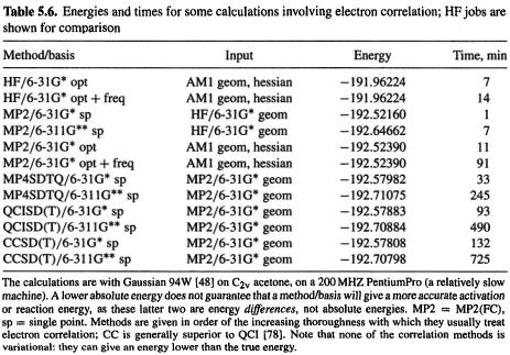
Instead of the very demanding CCSDT calculations one often performs CCSD(T) (note the parentheses), in which the contribution of triple excitations is represented in an approximate way (not refined iteratively); this could be called coupled cluster perturbative triples. The quadratic configuration method (QCI) is very similar to the CC method. The most accurate implementation of this in common use is QCISD(T) (quadratic CI singles, doubles, triples, with triple excitations treated in an approximate, non-iterative way). The CC method, which is usually only moderately slower than QCI (Table 5.6), is apparently better [78].
Like MP methods, CI methods require reasonably large basis sets for good results. The smallest (and perhaps most popular) basis used with these methods is the 6-31G*
Ab initio calculations 249
basis, but where practical the 6-311G** basis, developed especially for post-HF calculations, might be preferable (see Table 5.6). Higher-correlated single-point calculations on MP2 geometries tend to give more reliable energies relative energies than do singlepoint MP2 calculations on HF geometries (section 5.4.2, in connection with Figs 5.20 and 5.21). There is some evidence that when a correlation method is already being used, one tends to get improved geometries by using a bigger basis set rather than by going to a higher correlation level [79]. Figure 5.21 shows the results of HF and MP2 methods applied to chemical reactions. The limitations and advantages of numerous such methods are shown in a practical way in the Gaussian 94 workbook by Foresman and Frisch [1e]. Energies and times for some correlated calculations are given in Table 5.6.
Size-consistency
Two factors that should be mentioned in connection with post-HF calculations are the questions of whether a method is size-consistent and whether it is variational. A method is size-consistent if it gives the energy of a collection of n widely-separated atoms or molecules as being n times the energy of one of them. For example, the HF method gives the energy of two water molecules 20 Å apart (considered as a single system or “supermolecule”) as being twice the energy of one water molecule. The example below gives the result of HF/3-21G geometry optimizations on a water molecule, and on two water molecules at increasing distances (with the  supermolecule the O/H internuclear distance r was held constant at 10, 15,... Å while all the other geometric
250 Computational Chemistry
parameters were optimized):
As the two water molecules are separated a hydrogen bond (equilibrium bond length r = ca. 2.0 Å) is broken and the energy rises, levelling off at 20–25 Å to twice the energy of one water molecule. With the HF method we find that for any number n of molecules M, at large separation the energy of a supermolecule  equals n times the energy of one M. The HF method is thus size-consistent. A size-consistent method, we see, is one that scales in a way that makes sense.
Now, it is hard to see why, physically, the energy of n identical molecules so widelyseparated that they cannot affect one another should not be n times the energy of one molecule. Any mathematical method that does not mimic this physical behaviour would seem to have a conceptual flaw, and in fact lack of size-consistency also places limits on the utility of the program. For instance, in trying to study the hydrogenbonded water dimer we would not be able to equate the decrease in energy (compared to twice the energy of one molecule) with stabilization due to hydrogen bonding, and it is unclear how we could computationally turn off hydrogen bonding and evaluate the size-consistency error separately (actually, there is a separate problem, basis set superposition error – see below – with species like the water dimer, but this source of error can be dealt with). It might seem that any computational method must be sizeconsistent (why shouldn’t the energy of a large-separation  come out at n times that of M?). However, it is not hard to show that “straightforward” CI is not size-consistent unless Eqs (5.168) include all possible determinants, i.e. unless it is full CI. Consider a CISD calculation with a very large (“infinite”) basis set on two helium atoms which are separated by a large (“infinite”; say ca. 20Å) distance, and are therefore noninteracting. Note that although helium atoms do not form covalent
  molecules, at short distances they do interact to form van der Waals molecules. The wavefunction for this four-electron system will contain, besides the HF determinant, only determinants with single and double excitations (CISD). Lacking triple and quadruple excitations it will not produce the exact energy of our He–He system, which must be twice that of one helium atom, but instead will yield a higher energy. Now, a CISD calculation with an infinite basis set on a single He atom will give the exact wavefunction, and thus the exact energy of the atom (because only single and double promotions are possible for

Ab initio calculations 251
a two-electron system). Thus the energy of the infinitely-separated He–He system is not twice the energy of a single He atom in this calculation.
Variational behavior
The other factor to be discussed in connection with post-HF calculations is whether a particular method is variational. A method is variational (see the variation theorem, section 5.2.3.3) if any energy calculated from it is not less than the true energy of the electronic state and system in question, i.e if the calculated energy is an upper bound to the true energy. Using a variational method, as the basis set size is increased we get lower and lower energies, levelling off above the true energy (or at the true energy in the unlikely case that our method treats perfectly electron correlation, relativistic effects, and any other minor effects). Figure 5.18 shows that the calculated energy of using the HF method approaches a limit (–1.133…h) with increasingly large basis sets. The calculated energy can be lowered by using a correlated method and an adequate basis: full CI with the very big 6-311 + +G(3df, 3p2d) basis gives –1.17288 h, only
  (small compared with the H–H bond energy of
  above the accepted exact energy of –1.17439 h (Fig. 5.18).
If we cannot have both, it is more important for a method to be size-consistent than variational. Recall the methods we have seen in this book:
Hartree-Fock
MP (MP2, MP3, MP4, etc.)
full CI
truncated CI: CIS, CISD, etc.
MCSCF and its CASSCF variant
CC and its QCI variants (QCISD, QCISD(T), QCISDT, etc.)
The HF and full CI methods are both size-consistent and variational. All the other methods we have discussed are size-consistent but not variational. Thus we can use these methods to compare the energies of, say, water and the water dimer, but only with the HF or full CI methods can we be sure that the calculated energy is an upper bound to the exact energy, i.e. that the exact energy is really lower than the calculated (only a very high correlation level and basis set are likely to give essentially the exact energy; see section 5.5.2).
Basis set superposition error, BSSE
This is not associated with a particular method, like HF or CI, but rather is a basis set problem. Consider what happens when we compare the energy of the hydrogenbonded water dimer with that of two noninteracting water molecules. Here is the result of an MP2(FC)/6-31G* calculation; both structures were geometry-optimized, and the energies are corrected for ZPE:

252 Computational Chemistry
The straightforward conclusion is that at the MP2(FC)6-31G* level the dimer is stabler than two noninteracting water molecules by  If there are no other significant intermolecular forces, then we might say the H-bond energy in the water dimer [80] is
  (that it takes this energy to break the bond – to separate the dimer into noninteracting water molecules). Unfortunately there is a problem with this simple subtraction approach to comparing the energy of a weak molecular association AB with the energy of A plus the energy of B. If we do this we are assuming that if there were no interactions at all between A and B at the geometry of the AB species, then the AB energy would be that of isolated A plus that of isolated B. The problem is that when we do a calculation on the AB species (say the dimer
  in this “supermolecule” the basis functions (“atomic orbitals”) of B are available to A so A in AB has a bigger basis set than does isolated A; likewise B has a bigger basis than isolated B. When in AB each of the two components can borrow basis functions from the other. The error arises from “imposing” B’s basis set on A and vice versa, hence the name basis set superposition error. Because of BSSE A and B are not being fairly compared with AB, and we should use for the energies of separated A and of B lower values than we get in the absence of the borrowed functions. A little thought shows that accounting for BSSE will give a smaller value for the hydrogen bond energy (or van der Waals’ energy, or dipole–dipole attraction energy, or whatever weak interaction is being studied) than if it were ignored.
There are two ways to deal with BSSE. One is to say, as we implied above, that we should really compare the energy of AB with that of A with the extra basis functions provided by B, plus the energy of B with the extra basis functions provided by A. This method of correcting the energies of A and B with extra functions is called the counterpoise method [81], presumably because it balances (counterpoises) functions in A and B against functions in AB. In the counterpoise method the calculations on the components A and B of AB are done with ghost orbitals, which are basis functions (“atomic orbitals”) not accompanied by atoms (spirits without bodies, one might say): one specifies for A, at the positions that would be occupied by the various atoms of B in AB, atoms of zero atomic number bearing the same basis functions as the real atoms of B. This way there is no effect of atomic nuclei or extra electrons on A, just the availability of B’s basis functions. Likewise one uses ghost orbitals of A on B. A detailed description of the use of ghost orbitals in Gaussian 82 has been given by Clark [81a]. The counterpoise correction gives only an approximate value of the BSSE, and it is rarely applied to anything other than weakly-bound dimers, like hydrogen-bonded and van der Waals species: strangely, the correction worsens calculated atomization
energies (e.g. covalent |
and it is not uniquely defined for species of |
more than two components [81b]. |
|
The second way to handle BSSE is to swamp it with basis functions. Ifeach fragment A and B is endowed with a really big basis set, then extra functions from the other fragment won’t alter the energy much – the energy will already be near the asymptotic limit. So if one simply (!) carries out a calculation on A, B and AB with a sufficiently big basis, the straightforward procedure of subtracting the energy of AB from that of A + B should give a stabilization energy essentially free of BSSE. For good results one needs good geometries and adequate accounting for correlation effects. The use of large basis sets and high correlation levels to get high-quality atomization energies