


Ab initio calculations 281
atomization, because of the ability of isodesmic and related processes to compensate for basis set and correlation deficiencies (section 5.5.2.2a). In concluding our discussion of heats of formation, note that all these calculations of the heat of formation of methanol were not purely ab initio (quite apart from the empirical correction term in G2), since they required experimental values of either the heat of atomization of graphite (atomization and formation methods) or the heat of formation of methane (formation method). The inclusion of experimental values makes the calculation of heat of formation with the aid of ab initio methods a semiempirical procedure (do not confuse the term as used here with semiempirical programs like AM1, discussed in chapter 6). Augmentation with experimental data is needed whenever an ab initio calculation would involve an extended, solid substance like graphite (see the discussion in connection with the atomization method); other examples are phosphorus and sulfur.
Considerable attention has been given here to heats (enthalpies) of formation, because there are extensive tabulations of these [130] and papers on their calculation appear often in the literature [131]. However, we should remember that equilibria [103] are dependent not just on enthalpy differences, but also on the often-ignored entropy changes, as reflected in free energy differences, and so the calculation of entropies is also important [132].
5.5.2.3a Kinetics; calculating reaction rates
Ab initio kinetics calculations are far more challenging than thermodynamics calculations; in other words, the calculation of rate constants is much more involved than that of equilibrium constants or quantities like reaction enthalpy, reaction free energy, and heat of formation, which are related to equilibrium constants. Why is this so? After all, both rates and equilibria are related to the energy difference between two species: the rate constant to that between the reactant and transition state (TS), and the equilibrium constant to that between the reactant and product (Fig. 5.25). Furthermore, the energies of transition states, like those of reactants and products, can be calculated. The reason for the difference is partly because the energies of transition states are harder to calculate to high accuracy than are those of relative minima (“stable species”). Another problem is that the rate does not depend strictly on the TS/reactant free energy difference (which can, at sufficiently high levels, be accurately calculated).
To understand the problem consider a unimolecular reaction |
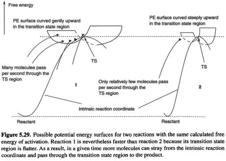
Figure 5.29 |
shows the potential energy surface for two reactions of this type, |
and |
 The reactions have identical calculated free energies of activation. By calculated, we mean here using some computational chemistry method (e.g. ab initio) and locating a stationary point with no imaginary frequencies, corresponding to A, and an appropriate stationary point with one imaginary frequency, etc. (section 2.5), corresponding to B. The “traditional” calculated rate constant then follows from a standard expression involving from the energy difference between the TS and reactant (our calculated free energy of activation) and the partition functions of the two species. However, in the TS region the PES for the first process is flatter than for the second process – the saddleshaped portion of the surface is less steeply-curved for reaction 1 than for reaction 2. If all reacting A molecules followed exactly the intrinsic reaction coordinate (IRC; section 2) and passed through the calculated TS species, then we might expect the two
282 Computational Chemistry
reactions to proceed at exactly the same rate, since all  and
and  molecules would have to surmount identical barriers. However, the IRC is only an idealization [133], and molecules passing through the TS region toward the product frequently stray from this path (dashed lines). Clearly for the reaction
  at any finite temperature more molecules (reflected in a Boltzmann distribution) will have the extra energy needed to traverse the higher-energy regions of the saddle, away from the TS point, than in the case of
 ifthe saddle were curved infinitely steeply, no molecules could stray outside the reaction path. Thus reaction 1 must be faster than reaction 2, although they have identical computed free energies ofactivation; the rate constant for reaction 1 must be bigger than that for reaction 2. The difficulty of obtaining good rate constants from accurate calculations on just two PES points, the reactant and the TS, is mitigated by this fact: the vibrational frequencies of the TS sample the curvature of the saddle region both along the reaction path (this curvature is represented by the imaginary frequency) and at “right angles” to the reaction path (represented by the other frequencies). High frequencies correspond to steep curvature. So when we use the TS frequencies in the partition function equation for the rate constant we are, in a sense, exploring regions of the PES saddle other than just the stationary point. The role of the curvature of the PES in affecting reaction rates is nicely alluded to by Cremer, who also shows the place of partition functions in rate equations [134].
Another way to calculate rates is by molecular dynamics [135]. Molecular dynamics calculations use the equations of classical physics to simulate the motion of a molecule under the influence of forces; the required force fields can be computed by ab initio methods or, for large systems, semiempirical methods (chapter 6) or molecular mechanics (chapter 3). In a molecular dynamics simulation of the reaction  molecules
Ab initio calculations 283
of A are “shaken” out of their potential well, and some pass through the saddle region at a rate that, for a given temperature, depends on the height of this region and its curvature. The height and curvature can be handled as an analytic function of atomic coordinates  which has been fitted to a finite number of calculated (e.g. by ab initio methods) points. The situation is even more complicated, because the simulation technique just outlined ignores quantum mechanical tunnelling [136], which, particularly where light atoms like hydrogen move, can speed up a reaction by orders of magnitude compared to classical predictions.
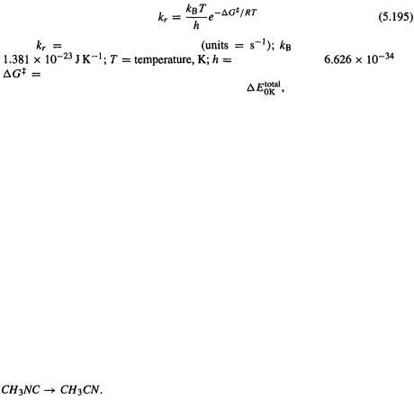
For rigorous calculations of rate constants one best utilizes specialized programs [137]. There are many discussions of the theory of reaction rates, in various degrees of detail [138]. In this section we will limit ourselves to gas-phase unimolecular reactions [139] and examine the results of some rough calculations. We will use the equation
where |
unimolecular rate constant |
= Boltzmann constant, |
|
|
Planck’s constant, |
J s; |
|
|
the transition-state-reactant free energy difference (in some calculations we |
||
will try the ZPE-corrected 0 K energy difference, |
which is the 0 K enthalpy |
||
difference); R = gas constant, 
This is not a rigorous equation for the unimolecular rate constant (which has highand low-pressure limiting forms anyway [139]). Roughly, Eq. (5.195) results from assuming that the rotational and vibrational partition functions do not change on going from the reactant to the TS in the high-pressure limit [140]; rates at the low-pressure limit appear to be slower than those at the high-pressure limit by a factor of roughly 1000 [141], In comparing calculated and experimental rate constants, we will consider the conditions to be the high-pressure limit (ca. 100mmHg or 13000Pa [141]. In the following calculations we will see if Eq. (5.195) is useful.
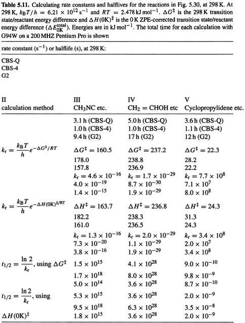
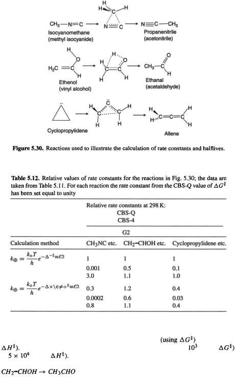
Consider the reactions in Fig. 5.30. Reactant and product structures were created with Spartan [30] and transition states were generated with Spartan’s transition state routine; semiempirical AM1 geometries from Spartan were used as input to G94W [48] CBS-Q, CBS-4 and G2 (section 5.5.2.2b) calculations. The results of the calculations are summarized in Tables 5.11 and 5.12. Table 5.12 shows that for a given reaction we got the same result, to within a factor of 10, whether we used CBS-Q or G2,  or
or  the biggest deviation is for
  a factor of 3.0 cf. 0.3. The CBS-4 method gave rate constants that are smaller than the CBS-Q and G2 rate constants by factors of from about 2
  to 5000
  using
using  These results may be compared with the experimental facts:
The experimental rate constant for the isocyanomethane (methyl isocyanide) to propanenitrile (acetonitrile) reaction is  at 298 K [142]. This compares astonishingly well with the value of
  in Table 5.11, calculated from the G2 value of
  the calculated rate constant is only a factor of three too small (using G2 with
  gives a rate constant too small by a factor of ten). The CBS-Q
284 Computational Chemistry

286 Computational Chemistry
The reported halflife of ethenol (vinyl alcohol) in the gas phase at room temperature is ca. 30min [143], far shorter than our calculated  However, the 30 min halflife is very likely that for a protonation/deprotonation isomerization catalyzed by the walls of the vessel, rather than for the concerted hydrogen migration (Fig. 5.30) considered here. Indeed, the related ethynol has been detected in planetary atmospheres and interstellar space [144], showing that that molecule, in isolation, is long-lived. All three methods predict very long halflives, the same to within a factor of two, regardless of whether one uses
  or
or 
Cyclopropylidene to allene
Cyclopropylidene has never been detected [145], so its halflife must be very short even well below room temperature. Our calculations predict room temperature halflives for
Cyclopropylidene |
Gaussian 94 and 98 can be instructed to calculate G |
||
(and H) at temperatures other than 298.15 K, so that |
and |
and thus equilibrium |
|
and rate constants, could be calculated for other temperatures, but if we just use the
298 K value of |
which should not change dramatically with temperature (cf. |
and |
in Table 5.11), we can estimate the halflife at 77 K |
(attempts to generate Cyclopropylidene at 77 K gave allene [146]). Equation (5.195) gives a halflife at 77 K of 590 s (10 min). Since this could easily be out by a factor of 10, the calculation accords with experiment. Cyclopropylidene should be easily observable at 10K, a routine matrix isolation [147] working temperature, where its halflife is calculated to be ca. 
These experimental facts and the comparison of the three computational methods suggest these tentative generalizations: the use of Eq. (5.195) with CBS-Q or (preferably?) G2 values of  gives for unimolecular isomerizations rate constants that are qualitatively reliable. The CBS-4 rate constants are smaller than the CBS-Q and G2 ones by a factor of from 2 to 1000. This is not bad for CBS-Q and G2, considering that Eq. (5.195) is quite approximate, and that the CBS and G2 methods (section 5.5.2.2b) were developed to provide reliable thermodynamic data, not to handle transition states.
From Eq. (5.195) and the fact that for a unimolecular reaction  follows that
At 298 K (about room temperature) this becomes
where |
is in |
|
|
Equation (5.196) shows that for |
is |
(at 10- |
|
298 K); this is |
about as expected, since the period of a molecular vibration is |
about |
s |
and with no barrier a species should survive for only about one |
vibra- |
tional motion (that along the reaction coordinate, corresponding to the imaginary frequency) as it passes through the saddle region (e.g. Fig. 5.29). Figure 5.31, a graph of Eq. (5.197), can be used to estimate halflives at room temperature from the free energy of activation, for unimolecular isomerizations. We see that the threshold value
of |
for observability at room temperature for a species that decays by a unimole- |
|
cular process is predicted to be roughly |
or 9 min), with |
|