

- •COMPUTATIONAL CHEMISTRY
- •CONTENTS
- •PREFACE
- •1.1 WHAT YOU CAN DO WITH COMPUTATIONAL CHEMISTRY
- •1.2 THE TOOLS OF COMPUTATIONAL CHEMISTRY
- •1.3 PUTTING IT ALL TOGETHER
- •1.4 THE PHILOSOPHY OF COMPUTATIONAL CHEMISTRY
- •1.5 SUMMARY OF CHAPTER 1
- •REFERENCES
- •EASIER QUESTIONS
- •HARDER QUESTIONS
- •2.1 PERSPECTIVE
- •2.2 STATIONARY POINTS
- •2.3 THE BORN–OPPENHEIMER APPROXIMATION
- •2.4 GEOMETRY OPTIMIZATION
- •2.6 SYMMETRY
- •2.7 SUMMARY OF CHAPTER 2
- •REFERENCES
- •EASIER QUESTIONS
- •HARDER QUESTIONS
- •3.1 PERSPECTIVE
- •3.2 THE BASIC PRINCIPLES OF MM
- •3.2.1 Developing a forcefield
- •3.2.2 Parameterizing a forcefield
- •3.2.3 A calculation using our forcefield
- •3.3 EXAMPLES OF THE USE OF MM
- •3.3.2 Geometries and energies of polymers
- •3.3.3 Geometries and energies of transition states
- •3.3.4 MM in organic synthesis
- •3.3.5 Molecular dynamics and Monte Carlo simulations
- •3.4 GEOMETRIES CALCULATED BY MM
- •3.5 FREQUENCIES CALCULATED BY MM
- •3.6 STRENGTHS AND WEAKNESSES OF MM
- •3.6.1 Strengths
- •3.6.2 Weaknesses
- •3.7 SUMMARY OF CHAPTER 3
- •REFERENCES
- •EASIER QUESTIONS
- •HARDER QUESTIONS
- •4.1 PERSPECTIVE
- •4.2.1 The origins of quantum theory: blackbody radiation and the photoelectric effect
- •4.2.2 Radioactivity
- •4.2.3 Relativity
- •4.2.4 The nuclear atom
- •4.2.5 The Bohr atom
- •4.2.6 The wave mechanical atom and the Schrödinger equation
- •4.3.1 Introduction
- •4.3.2 Hybridization
- •4.3.3 Matrices and determinants
- •4.3.4 The simple Hückel method – theory
- •4.3.5 The simple Hückel method – applications
- •4.3.6 Strengths and weaknesses of the SHM
- •4.4.1 Theory
- •4.4.2 An illustration of the EHM: the protonated helium molecule
- •4.4.3 The extended Hückel method – applications
- •4.4.4 Strengths and weaknesses of the EHM
- •4.5 SUMMARY OF CHAPTER 4
- •REFERENCES
- •EASIER QUESTIONS
- •5.1 PERSPECTIVE
- •5.2.1 Preliminaries
- •5.2.2 The Hartree SCF method
- •5.2.3 The HF equations
- •5.2.3.1 Slater determinants
- •5.2.3.2 Calculating the atomic or molecular energy
- •5.2.3.3 The variation theorem (variation principle)
- •5.2.3.4 Minimizing the energy; the HF equations
- •5.2.3.5 The meaning of the HF equations
- •5.2.3.6a Deriving the Roothaan–Hall equations
- •5.3 BASIS SETS
- •5.3.1 Introduction
- •5.3.2 Gaussian functions; basis set preliminaries; direct SCF
- •5.3.3 Types of basis sets and their uses
- •5.4 POST-HF CALCULATIONS: ELECTRON CORRELATION
- •5.4.1 Electron correlation
- •5.4.3 The configuration interaction approach to electron correlation
- •5.5.1 Geometries
- •5.5.2 Energies
- •5.5.2.1 Energies: Preliminaries
- •5.5.2.2 Energies: calculating quantities relevant to thermodynamics and to kinetics
- •5.5.2.2a Thermodynamics; “direct” methods, isodesmic reactions
- •5.5.2.2b Thermodynamics; high-accuracy calculations
- •5.5.2.3 Thermodynamics; calculating heats of formation
- •5.5.2.3a Kinetics; calculating reaction rates
- •5.5.2.3b Energies: concluding remarks
- •5.5.3 Frequencies
- •Dipole moments
- •Charges and bond orders
- •Electrostatic potential
- •Atoms-in-molecules
- •5.5.5 Miscellaneous properties – UV and NMR spectra, ionization energies, and electron affinities
- •5.5.6 Visualization
- •5.6 STRENGTHS AND WEAKNESSES OF AB INITIO CALCULATIONS
- •5.7 SUMMARY OF CHAPTER 5
- •REFERENCES
- •EASIER QUESTIONS
- •HARDER QUESTIONS
- •6.1 PERSPECTIVE
- •6.2 THE BASIC PRINCIPLES OF SCF SE METHODS
- •6.2.1 Preliminaries
- •6.2.2 The Pariser-Parr-Pople (PPP) method
- •6.2.3 The complete neglect of differential overlap (CNDO) method
- •6.2.4 The intermediate neglect of differential overlap (INDO) method
- •6.2.5 The neglect of diatomic differential overlap (NDDO) method
- •6.2.5.2 Heats of formation from SE electronic energies
- •6.2.5.3 MNDO
- •6.2.5.7 Inclusion of d orbitals: MNDO/d and PM3t; explicit electron correlation: MNDOC
- •6.3 APPLICATIONS OF SE METHODS
- •6.3.1 Geometries
- •6.3.2 Energies
- •6.3.2.1 Energies: preliminaries
- •6.3.2.2 Energies: calculating quantities relevant to thermodynamics and kinetics
- •6.3.3 Frequencies
- •6.3.4 Properties arising from electron distribution: dipole moments, charges, bond orders
- •6.3.5 Miscellaneous properties – UV spectra, ionization energies, and electron affinities
- •6.3.6 Visualization
- •6.3.7 Some general remarks
- •6.4 STRENGTHS AND WEAKNESSES OF SE METHODS
- •6.5 SUMMARY OF CHAPTER 6
- •REFERENCES
- •EASIER QUESTIONS
- •HARDER QUESTIONS
- •7.1 PERSPECTIVE
- •7.2 THE BASIC PRINCIPLES OF DENSITY FUNCTIONAL THEORY
- •7.2.1 Preliminaries
- •7.2.2 Forerunners to current DFT methods
- •7.2.3.1 Functionals: The Hohenberg–Kohn theorems
- •7.2.3.2 The Kohn–Sham energy and the KS equations
- •7.2.3.3 Solving the KS equations
- •7.2.3.4a The local density approximation (LDA)
- •7.2.3.4b The local spin density approximation (LSDA)
- •7.2.3.4c Gradient-corrected functionals and hybrid functionals
- •7.3 APPLICATIONS OF DENSITY FUNCTIONAL THEORY
- •7.3.1 Geometries
- •7.3.2 Energies
- •7.3.2.1 Energies: preliminaries
- •7.3.2.2 Energies: calculating quantities relevant to thermodynamics and kinetics
- •7.3.2.2a Thermodynamics
- •7.3.2.2b Kinetics
- •7.3.3 Frequencies
- •7.3.6 Visualization
- •7.4 STRENGTHS AND WEAKNESSES OF DFT
- •7.5 SUMMARY OF CHAPTER 7
- •REFERENCES
- •EASIER QUESTIONS
- •HARDER QUESTIONS
- •8.1 FROM THE LITERATURE
- •8.1.1.1 Oxirene
- •8.1.1.2 Nitrogen pentafluoride
- •8.1.1.3 Pyramidane
- •8.1.1.4 Beyond dinitrogen
- •8.1.2 Mechanisms
- •8.1.2.1 The Diels–Alder reaction
- •8.1.2.2 Abstraction of H from amino acids by the OH radical
- •8.1.3 Concepts
- •8.1.3.1 Resonance vs. inductive effects
- •8.1.3.2 Homoaromaticity
- •8.2 TO THE LITERATURE
- •8.2.1 Books
- •8.2.2 The Worldwide Web
- •8.3 SOFTWARE AND HARDWARE
- •8.3.1 Software
- •8.3.2 Hardware
- •8.3.3 Postscript
- •REFERENCES
- •INDEX
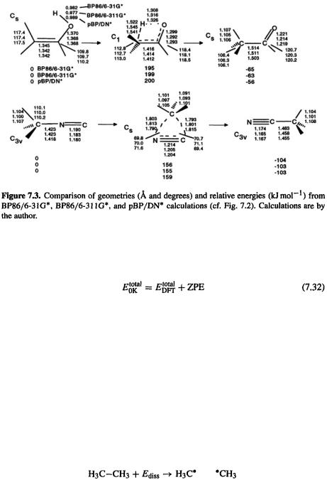
Density Functional Calculations 407
repulsion. In accurate work this “raw” energy should be corrected by adding the zeropoint vibrational energy, to obtain the total internal energy at 0 K. Analogously to the HF equation in section 5.2.3.6d, Eq. (94) we have
(The Gaussian programs actually denote the DPT energy called here  as HF, e.g. (in hartrees or atomic units)
  The main advantage of DFT over HF calculations is in being able to provide, in a comparable time, superior energy-difference results (reaction energies, activation energies, and electronic transition energies, i.e. UV spectra). We concentrate on energies from B3LYP/6-31G* and pBP/DN* calculations for the same reasons that these two methods were chosen for the geometry calculations in section 7.3.1.
7.3.2.2Energies: calculating quantities relevant to thermodynamics and kinetics
7.3.2.2a Thermodynamics
Let us first see how DFT handles a case where HF fails badly: homolytic breaking of a covalent bond (section 5.4.1). Consider the reaction
In principle, the dissociation energy can be found simply as the energy of two methyl radicals minus the energy of ethane. Table 7.3 (cf. Table 5.5) shows the results of  and two
  and pBP) calculations.
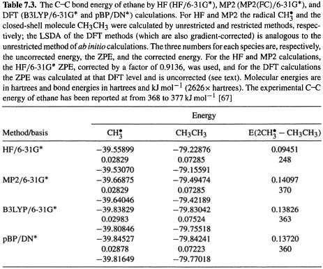
408 Computational Chemistry
The HF and MP2 ZPEs are from HF/6-31G* optimizations/frequency jobs, and were corrected by multiplying by 0.9136 [62]; the DFT ZPEs are from the B3LYP/6-3G* and pBP optimizations/frequencies and are uncorrected, since the correction factor should be close to unity [62]. As we saw in chapter 5, the HF method gives a very poor estimate of the bond energy, while the MP2 calculation provides a good value. Here we see that the B3LYP and pBP methods give a bond energy only slightly less than that from the MP2 calculation. Note, however, that in general, to get good (reliably within 10 or even  atomization energies and reaction energies simply by subtraction requires "high-accuracy” methods, using higher-level electron correlation and bigger basis sets (section 5.5.2.2b). Martell et al. tested six functionals on 44 atomization energies and six reactions and concluded that the best atomization energies were obtained with hybrid functionals, but slightly better reaction enthalpies were obtained with non-hybrid ones [63]. St.-Amant et al. found that gradient-corrected functionals gave good geometries and energies for conformers; the dihedrals were on average within 4° of experiment and the relative energies were nearly as accurate as those from MP2 [56]. Scheiner et al. found that, as for geometries, Becke’s original three-parameter function (usually called ACM, adiabatic connection method) gave the best reaction energies [55].
Density Functional Calculations 409
410 Computational Chemistry
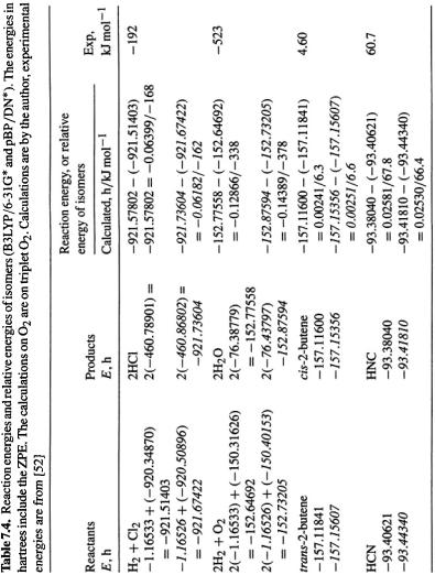
Some reaction energies and relative energies of isomers are compared in Table 7.4 (cf. Table 5.9, Table 6.3).The results for the HCl and  formation reactions show no particular improvement over the HF calculations in Table 5.9. The 2-butene cis/trans energy difference error is about the same, but the HCN/HNC energy difference is closer to the experimental value. A large number of energy difference comparisons have been published for the pBP/DN* and pBP/DN** methods cf. HF, MP2 and experiment [48], and for B3LYP/6-31G* methods compared to HF, MP2 and experiment [52]. These comparisons involve homolytic dissociation, various reactions particularly hydrogenations, acid–base reactions, isomerizations, isodesmic reactions, and conformational energy differences. This wealth of data shows that while gradient-corrected DFT and MP2 calculations are vastly superior for homolytic dissociations, for “ordinary” reactions (involving only closed-shell species), their advantage is much less marked; for example, HF/3-21G, HF/6-31G*. SVWN/6-31G* (non-gradient-corrected DFT), all usually give energy differences similar to those from B3LYP/6-31G* and pBP/DN* and in fair agreement with experiment. Table 7.5 compares errors for hydrogenations, isomerizations, bond separation reactions (a kind of isodesmic reaction), and proton affinities; the methods are HF, SVWN, MP2, and B3LYP, all using the 6-31G* basis. In two of the four cases (hydrogenation and isomerization) the HF/6-31G* method gave the best results; in one case MP2 was best and in one case B3LYP. For the energy comparison of normal (not involving transition states) closed-shell organic species correlated methods like MP2 and DFT seem to offer little or no advantage, unless one needs accuracy within ca.
  of experiment, in which case high-accuracy methods should be used. The strength of gradient-corrected DFT methods appears to lie largely in their ability to give homolytic dissociation energies and activation energies with an accuracy comparable to that from MP2, but at a time cost comparable to that from HF calculations.
Bauschlicher et al. compared various methods and recommended B3LYP over HF and MP2, to a large extent on the basis of the performance of B3LYP with regard to atomization energies and transition metal compounds [58]. Wiberg and Ochterski compared HF, MP2, MP3, MP4, B3LYP, CBS-4 and CBS-Q with experiment in calculating energies of isodesmic reactions (hydrogenation and hydrogenolysis, hydrogen transfer, isomerization, and carbocation reactions) and found that while MP4/6-31G* and CBS- Q were the best, B3LYP/6-31G* was also generally satisfactory [64]. Rousseau and