

Ab initio calculations 287
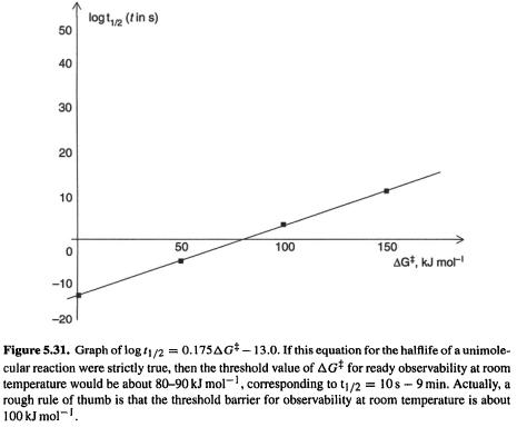
a strong dependence on  Experience shows that in fact the threshold barrier for observing or isolating a compound at room temperature is about
5.5.2.3b Energies: concluding remarks
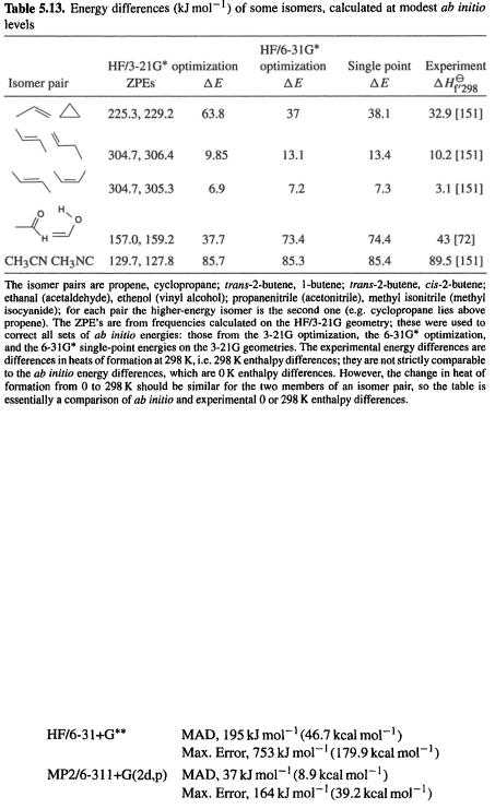
Although we have paid considerable attention to high-accuracy energy methods (CBS and G2), many ab initio studies are limited to obtaining relative energies at a moderate level like MP2/6-31G*, or even HF/6-31G* or HF/3-21G. In comparing the thermodynamic stabilities of isomers (in contrast to calculating an “absolute” thermodynamic parameter like the heat of formation of a compound), simple subtraction of ab initio energies calculated at a modest level (e.g. Fig. 5.24) usually gives at least semiquantitatively reliable results. Some examples of energy differences calculated at modest ab initio levels are shown in Table 5.13. Here  (section 5.2.3.6d), the ZPE-corrected ab initio energy, has been used to calculate energy differences for five pairs of isomers. The ab initio energies are from HF/3-21G-optimized geometries, HF/6-31G*-optimized geometries, and single-point HF/6-31G* calculations on HF/3- 21G-optimized geometries; the ZPE corrections are all from HF/3-21G* frequencies on HF/3-21G-optimized geometries. Although ZPE corrections have been included here, ignoring them for such modest-level calculations on pairs of isomers evidently makes little difference, as the correction is the same for both isomers, to within a few
(but for comparison of a ground state and a TS the ZPE correction is more likely to be significant, see e.g. Fig. 2.20; and in high-accuracy calculations ZPE’s should always
288 Computational Chemistry
be included). This very small sample does not permit one to draw conclusions about  energies, but this has been discussed in sections 5.3.3 and 5.5.2.2a. The single-point
  energies are almost identical to the optimized-geometry ones (correlated single-point energies were discussed in sections 5.4.2 and 5.4.3). Agreement with experiment (the 0 and 298 K enthalpy values are approximately comparable) is good except for ethanal/ethenol; the reported experimental value of
  for this pair is supported by a high-accuracy energy calculation (CBS-Q, section 5.5.2.2b) that gives a 0 K enthalpy difference of
  at 298 K, bolstering the assertion that
  changes little from 0 to 298 K). The two
  values are evidently in error by about
  while the
  error is only
  A “higher” level is not guaranteed to give more accurate results, at least not until we reach very high levels. As might be suspected, the relative energies of conformers is also treated quite well by these modest levels [148].
Foresman and Frisch [149], in a chapter with very useful data and recommendations, show large mean absolute deviations (MAD) and enormous maximum errors for HF and even MP2 methods; e.g.