

210 Computational Chemistry
small enough to be neglected (as is the case for functions on distant nuclei; this decreases
the time of a calculation from an |
dependence on the number of basis function to |
|
about an |
dependence); recalculating integrals to avoid the bottleneck of hard-drive |
|
access (direct SCF, section 5.3.2); representing the MOs as a set of gridpoints in space (in addition to a basis set expansion), which eliminates the need to explicitly calculate two-electron integrals. This pseudospectral method speeds up ab initio calculations by a factor of perhaps three or four. Methods of speeding up calculations are explained, with references to the literature, by Levine [27].
The method of calculating wavefunctions and energies that has been described in this chapter applies to closed-shell, ground-state molecules. The Slater determinant we started with (Eq. (5.12)) applies to molecules in which the electrons are fed pairwise into the MO’s, starting with the lowest-energy MO; this is in contrast to free radicals, which have one or more unpaired electrons, or to electronically excited molecules, in which an electron has been promoted to a higher-level MO (e.g. Fig. 5.9, neutral triplet). The HF method outlined here is based on closed-shell Slater determinants and is called the restricted HF method or RHF method; “restricted” means that the electrons of  spin are forced to occupy (restricted to) the same spatial orbitals as those of
 spin: inspection of Eq. (5.12) shows that we do not have a set of
  spatial orbitals and a set of
  spatial orbitals. If unqualified, a HF (i.e. an SCF) calculation means an RHF calculation.
The common way to treat free radicals is with the unrestricted HF method or UHF method. In this method, we employ separate spatial orbitals forthe and the
 electrons, giving two sets of MOs, one for
 and one for
 electrons. Less commonly, free radicals are treated by the restricted open-shell HF or ROHF method, in which electrons occupy MO’s in pairs as in the RHF method, except for the unpaired electron(s). The theoretical treatment of open-shell species is discussed in [1,10, l(k, l)], in particular, compare the performance of the UHF and ROHF methods.
Excited states, and those unusual molecules with electrons of opposite spin singly occupying different spatial MO’s (open-shell singlets) cannot be properly treated with a single-determinant wavefunction. They must be handled with approaches beyond the HF level, such as configuration interaction (section 5.4).
5.3BASIS SETS
5.3.1Introduction
We encountered basis sets in sections 4.3.3, and 4.4.1a, and 5.2.3.6a. A basis set is a set of mathematical functions (basis functions), linear combinations of which yield molecular orbitals, as shown in Eqs (5.51) and (5.52). The functions are usually, but not invariably , centered on atomic nuclei (Fig. 5.7). Approximating molecular orbitals as linear combinations ofbasis functions is usually called the LCAO or linear combination of atomic orbitals approach, although the functions are not necessarily conventional atomic orbitals: they can be any set of mathematical functions that are convenient to manipulate and which in linear combination give useful representations of MOs. With this reservation, LCAO is a useful acronym. Physically, several (usually) basis functions
Ab initio calculations 211
describe the electron distribution around an atom and combining atomic basis functions yields the electron distribution in the molecule as a whole. Basis functions not centered on atoms (occasionally used) can be considered to lie on “ghost atoms”; see basis set superposition error, section 5.4.3.
The simplest basis sets are those used in the SHM and EHM (chapter 4). As applied to conjugated organic compounds (its usual domain), the simple Hückel basis set consists of just p atomic orbitals (or “geometrically p-type” atomic orbitals, like a lone-pair orbital which can be considered not to interact with the  framework). The extended Hückel basis set consists of only the atomic valence orbitals. In the SHM, we do not worry about the mathematical form of the basis functions, reducing the interactions between them to 0 or –1 in the SHM Fock matrix (e.g. Eqs (4.62) and (4.64)). In the EHM the valence atomic orbitals are represented as Slater functions (section 4.4.1a).
5.3.2Gaussian functions; basis set preliminaries; direct SCF
The electron distribution around an atom can be represented in several ways. Hydrogenlike functions based on solutions of the Schrödinger equation for the hydrogen atom, polynomial functions with adjustable parameters, Slater functions (Eq. (5.95)), and Gaussian functions (Eq. (5.96)) have all been used [28]. Of these, Slater and Gaussian functions are mathematically the simplest, and it is these that are currently used as the basis functions in molecular calculations. Slater functions are used in semiempirical calculations, like the EHM (section 4.4) and other semiempirical methods (chapter 6). Modern molecular ab initio programs employ Gaussian functions.
Slater functions are good approximations to atomic wavefunctions and would be the natural choice for ab initio basis functions, were it not for the fact that the evaluation of certain two-electron integrals requires excessive computer time if Slater functions are used. The two-electron integrals (sections 5.2.3.6c, e) of the G matrix (Eq. (5.100)) involve four functions, which may be on from one to four centers (normally atomic nuclei). Those two-electron integrals with three or four different functions
 and
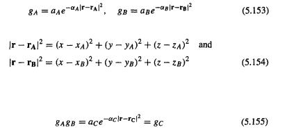
and  and three or four nuclei (threeor four-center integrals) are extremely difficult to calculate with Slater functions, but are readily evaluated with Gaussian basis functions. The reason is that the product of two Gaussians on two centers is a Gaussian on a third center. Consider an s-type Gaussian centered on nucleus A and one on nucleus B; we are considering real functions, which is what basis functions normally are:
where
with the nuclear and electron positions in Cartesian coordinates (ifthese were not s-type functions, the preexponential factor would contain one or more cartesian variables to give the function (the “orbital”) nonspherical shape). It is not hard to show that
212 Computational Chemistry |
|
|
||
The product of |
and |
is the Gaussian |
centered at |
Now consider the general |
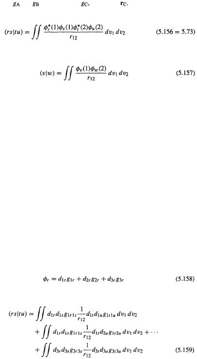
electron-repulsion integral |
|
|
||
If each basis function were a single, real Gaussian, then from Eq. (5.155) this would reduce to
i.e. threeand four-center two-electron integrals with four basis functions would immediately simplify to tractable two-center integrals with two functions.
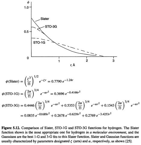
Actually, things are a little more complicated. A single Gaussian is a poor approximation to the nearly ideal description of an atomic wavefunction that a Slater function provides. Figure 5.12 shows that a Gaussian (designated STO-1G) is rounded near  while a Slater function has a cusp there (zero slope vs. a finite slope at
  the Gaussian also decays somewhat faster than the Slater function at large r. The solution to the problem of this poor functional behaviour is to use several Gaussians to approximate a Slater function. In Fig. 5.12 a single Gaussian and a linear combination of three Gaussians have been used to approximate the Slater function shown; the nomenclature STO-1G and STO-3G mean “Slater-type orbital (approximated by) one Gaussian” and “Slater-type orbital (approximated by) three Gaussians”, respectively. The Slater function shown is one suitable for a hydrogen atom in a molecule
  and the Gaussians are the best fit to this Slater function. STO-1G functions were used in our illustrative HF calculation on
 (section 5.2.3.6e), and the STO-3G function is the smallest basis function used in standard ab initio calculations by commercial programs. Three Gaussians are a good speed vs. accuracy compromise between two and four or more [25].
The STO-3G basis function in Fig. 5.12 is a contracted Gaussian consisting of three primitive Gaussians each of which has a contraction coefficient (0.4446, 0.5353 and 0.1543). Typically, an ab initio basis function consists of a set of primitive Gaussians bundled together with a set of contraction coefficients. Now consider the two-electron integral (Eq. (5.156)). Suppose each basis function is an STO-3G contracted Gaussian, i.e.
and analogously for  and
and  Then it is easy to see that
Ab initio calculations 213
where and so on. Thus with contracted Gaussians as basis functions, each two-electron integral becomes a sum of easily calculated two-center two-electron integrals. Gaussian integrals can be evaluated so much faster than Slater integrals that the use of contracted Gaussians instead of Slater functions speeds up the calculation of the integrals enormously, despite the larger number of integrals. Discussions of the number of integrals in an ab initio calculation usually refer to those at the contracted Gaussian level, rather than the greater number engendered by the use of primitive Gaussians; thus the program Gaussian 92 [23] says that both an STO-1G and an STO-3G calculation on water use the same number (144) of two-electron integrals, although the latter clearly involves more “primitive integrals.” The fruitful suggestion to use Gaussians in molecular calculations came from Boys (1950 [29]); it played a major role in making ab initio calculations practical, and this is epitomized in the names of the Gaussian series of programs, e.g. Gaussian 92 [23], which are possibly the most widely-used ab initio programs.
214 Computational Chemistry
Fast calculation of integrals is particularly important for the two-electron integrals, as their number increases rapidly with the size of the molecule and the basis set (basis sets are discussed in section 5.3.3). Consider a calculation on water with an STO1G basis set (and bear in mind that the smallest basis set normally used in ab initio calculations is the STO-3G set). In a standard ab initio calculation we use at least one basis function for each core orbital and each valence-shell orbital. Thus the oxygen
requiresfivebasis functions, forthe |
and |
orbitals; we can designate |
||
these functions |
anddenotethe 1shydrogenfunctions, one foreachH, |
|||
and |
In computational chemistry atoms beyond hydrogen and helium in the periodic |
|||
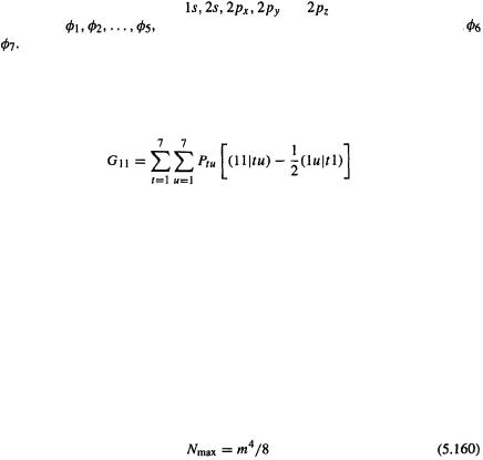
table are called “heavy atoms”, and the computational “first row” is lithium–neon. With experience, the number of heavy atoms in a molecule gives a quick indication of about how many basis functions will be invoked by a specified basis set. Following the procedure for  in Eq. (5.106):
Now u runs from 1 to 7 and t from 1 to 7, so  will consist of 49 terms, each containing two two-electron integrals for a
  total of 98 integrals. The Fock matrix for seven basis functions is a 7 × 7 matrix with 49 elements,
  so apparently there are 49 × 98 = 4802 two-electron integrals. Actually, many of these are duplicates(
 scan
scan Fock matrix has only about
 different elements), differ from other integrals only in sign, or are very small, and the number of unique nonvanishing two-electron integrals is 119 (calculated with Gaussian 92 [23]). For an STO-1G calculation on hydrogen peroxide (12 basis functions), there are ca. 700 unique nonvanishing two-electron integrals (cf. a naive theoretical maximum of 41472). The usual formula for estimating the maximum numberofunique two-electron integrals for a set of m real basis functions derives from the fact that there are four basis functions in each integral and
  is eightfold degenerate (Eq. (5.109)); this approximates the maximum number of these integrals as
In the above calculations the symmetry of water and hydrogen peroxide
 plays an important role in reducing the number of integrals which must actually be calculated, and modern ab initio programs recognize and utilize symmetry where it can be used (most molecules lack symmetry, but the small molecules ofparticular theoretical interest usually possess it), and are also able to recognize and avoid calculating integrals below a threshold size. Nevertheless the rapid rise in the number of 2-electron integrals with molecular and basis set size portends problems for ab initio calculations. An ab initio calculation on aspirin, a fairly small
  13 heavy atoms) molecule of practical interest, using the 3-21G basis set (section 5.3.3), which is the smallest that is usually used, requires 133 basis functions, which from Eq. (5.160) could invoke up to 39 million
 two-electron integrals. Clearly, a modest ab initio calculation could require tens of millions of integrals. Information on molecular size, symmetry, basis sets and number of integrals is summarized in Table 5.2 (the 3-21G basis set is

Ab initio calculations 215
explained in section 5.3.3). Note that for those molecules with no symmetry  the number of two-electron integrals calculated from Eq. (5.160) is about the same as that actually calculated by Gaussian 92.
There are two problems with so many two-electron integrals: the time needed to calculate them, and where to store them. Solutions to the first problem are, as explained, to use Gaussian functions, to utilize symmetry where possible, and to ignore those integrals that a preliminary check reveals are “vanishing”. The other problem can be dealt with by storing the integrals in the RAM (the random access memory, i.e. the electronic memory), storing the integrals on the hard drive, or not storing them at all, but rather calculating them as they are required. Calculating all the integrals at the outset and storing them somewhere is called conventional scf, being the earlierused procedure. The latter procedure of calculating only those two-electron integrals needed at the moment, and recalculating them again when necessary, is called direct scf (presumably using “direct” in the sense of “just now” or “at the moment”). Calculating all the two-electron the integrals and storing them in the RAM is the fastest approach, since it requires them to be calculated only once, and accessing information from the electronic memory is fast. However, RAM cannot yet store as many integrals as the hard drive. A (currently) respectable memory of 1GB can store all the integrals generated by perhaps about 1000 basis functions (up to about 50 million); beyond this the computer essentially grinds to a halt. The capacity of the hard drive is typically considerably greater than that of the RAM (say, 50 GB for a respectable hard drive), and storing all the two-electron integrals on the hard drive is often a viable option, but suffers from the disadvantage that the time taken to read data from a mechanical device like the hard drive into the RAM, where it can be used by the cpu, is much greater (perhaps a millisecond compared to a nanosecond) than the time needed to access the information were it stored in a purely electronic device like the RAM (which is the only alternative to direct scf in, e.g. Spartan [30]). For these reasons, ab initio calculations with many basis functions (beyond about 120, depending on the size of the RAM) nowadays use direct scf, despite the need to recalculate integrals [31]. These considerations will change with improvements in hardware, and the availability of very large electronic memories may make