17.2 Detailed Routing

The global routing step determines the channels to be used for each interconnect. Using this information the detailed router decides the exact location and layers for each interconnect. Figure 17.9 (a) shows typical metal rules. These rules determine the m1 routing pitch ( track pitch , track spacing , or just pitch ). We can set the m1 pitch to one of three values:

1.via-to-via ( VTV ) pitch (or spacing),

2.via-to-line ( VTL or line-to-via ) pitch, or

3.line-to-line ( LTL ) pitch.

The same choices apply to the m2 and other metal layers if they are present. Via-to-via spacing allows the router to place vias adjacent to each other. Via-to-line spacing is hard to use in practice because it restricts the router to nonadjacent vias. Using line-to-line spacing prevents the router from placing a via at all without using jogs and is rarely used. Via-to-via spacing is the easiest for a router to use and the most common. Using either via-to-line or via-to-via spacing means that the routing pitch is larger than the minimum metal pitch.

Sometimes people draw a distinction between a cut and a via when they talk about large connections such as shown in Figure 17.10 (a). We split or stitch a large via into identically sized cuts (sometimes called a waffle via ). Because of the profile of the metal in a contact and the way current flows into a contact, often the total resistance of several small cuts is less than that of one large cut. Using identically sized cuts also means the processing conditions during contact etching, which may vary with the area and perimeter of a contact, are the same for every cut on the chip.

In a stacked via the contact cuts all overlap in a layout plot and it is impossible to tell just how many vias on which layers are present. Figure 17.10 (b f) show an alternative way to draw contacts and vias. Though this is not a standard, using the diagonal box convention makes it possible to recognize stacked vias and contacts on a layout (in any orientation). I shall use these conventions when it is necessary.

FIGURE 17.9 The metal routing pitch. (a) An example of l -based metal design rules for m1 and via1 (m1/m2 via). (b) Via-to-via pitch for adjacent vias.

(c) Via-to-line (or line-to-via) pitch for nonadjacent vias. (d) Line-to-line pitch with no vias.

FIGURE 17.10 (a) A large m1 to m2 via. The black squares represent the holes (or cuts) that are etched in the insulating material between the m1 and 2 layers.

(b) A m1 to m2 via (a via1). (c) A contact from m1 to diffusion or polysilicon (a contact). (d) A via1 placed over (or stacked over) a contact. (e) A m2 to m3 via (a via2) (f) A via2 stacked over a via1 stacked over a contact. Notice that the black square in parts b c do not represent the actual location of the cuts. The black squares are offset so you can recognize stacked vias and contacts.

In a two-level metal CMOS ASIC technology we complete the wiring using the two different metal layers for the horizontal and vertical directions, one layer for each direction. This is Manhattan routing , because the results look similar to the rectangular north south and east west layout of streets in New York City. Thus, for example, if terminals are on the m2 layer, then we route the horizontal branches in a channel using m2 and the vertical trunks using m1. Figure 17.11 shows that, although we may choose a preferred direction for each metal layer (for example, m1 for horizontal routing and m2 for vertical routing), this may lead to problems in cases that have both horizontal and vertical channels. In these cases we define a preferred metal layer in the direction of the channel spine. In Figure 17.11 , because the logic cell connectors are on m2, any vertical channel has to use vias at every logic cell location. By changing the orientation of the metal directions in vertical channels, we can avoid this, and instead we only need

to place vias at the intersection of horizontal and vertical channels.

FIGURE 17.11 An expanded view of part of a cell-based ASIC. (a) Both channel 4 and channel 5 use m1 in the horizontal direction and m2 in the vertical direction. If the logic cell connectors are on m2 this requires vias to be placed at every logic cell connector in channel 4. (b) Channel 4 and 5 are routed with m1 along the direction of the channel spine (the long direction of the channel). Now vias are required only for nets 1 and 2, at the intersection of the channels.

Figure 17.12 shows an imaginary logic cell with connectors. Double-entry logic cells intended for two-level metal routing have connectors at the top and bottom of the logic cell, usually in m2. Logic cells intended for processes with three or more levels of metal have connectors in the center of the cell, again usually on m2. Logic cells may use both m1 and m2 internally, but the use of m2 is usually minimized. The router normally uses a simplified view of the logic cell called a phantom . The phantom contains only the logic cell information that the router needs: the connector locations, types, and names; the abutment and bounding boxes; enough layer information to be able to place cells without violating design rules; and a blockage map the locations of any metal inside the cell that blocks routing.

FIGURE 17.12 The different types of connections that can be made to a cell. This cell has connectors at the top and bottom of the cell (normal for cells intended for use with a two-level metal process) and internal connectors (normal for logic cells intended for use with a three-level metal process). The interconnect and connections are drawn to scale.

Figure 17.13 illustrates some terms used in the detailed routing of a channel. The channel spine in Figure 17.13 is horizontal with terminals at the top and the bottom, but a channel can also be vertical. In either case terminals are spaced along the longest edges of the channel at given, fixed locations. Terminals are usually located on a grid defined by the routing pitch on that layer (we say terminals are either on-grid or off-grid ). We make connections between terminals using interconnects that consist of one or more trunks running parallel to the length of the channel and branches that connect the trunk to the terminals. If more than one trunk is used, the trunks are connected by doglegs . Connections exit the channel at pseudoterminals .

FIGURE 17.13 Terms used in channel routing. (a) A channel with four horizontal tracks. (b) An expanded view of the left-hand portion of the channel showing (approximately to scale) how the m1 and m2 layers connect to the logic cells on either side of the channel. (c) The construction of a via1 (m1/m2 via).

The trunk and branch connections run in tracks (equispaced, like railway tracks). If the trunk connections use m1, the horizontal track spacing (usually just called the track spacing for channel routing) is equal to the m1 routing pitch. The maximum number of interconnects we need in a channel multiplied by the horizontal track spacing gives the minimum height of a channel (see

Section 17.2.2 on how to determine the maximum number of interconnects needed). Each terminal occupies a column . If the branches use m2, the column spacing (or vertical track spacing ) is equal to the m2 routing pitch.

17.2.1 Goals and Objectives

The goal of detailed routing is to complete all the connections between logic cells. The most common objective is to minimize one or more of the following:

●The total interconnect length and area

●The number of layer changes that the connections have to make

●The delay of critical paths

Minimizing the number of layer changes corresponds to minimizing the number of vias that add parasitic resistance and capacitance to a connection.

In some cases the detailed router may not be able to complete the routing in the

router uses only one trunk for each net. This restriction has the effect of minimizing the number of connections between the routing layers. This is equivalent to minimizing the number of vias used by the channel router in a two-layer metal technology. Minimizing the number of vias is an important objective in routing a channel, but it is not always practical. Sometimes constraints will force a channel router to use jogs or other methods to complete the routing (see Section 17.2.5 ). Next, though, we shall study an algorithm that solves the restricted channel-routing problem.

17.2.4 Left-Edge Algorithm

The left-edge algorithm ( LEA ) is the basis for several routing algorithms [ Hashimoto and Stevens, 1971]. The LEA applies to two-layer channel routing, using one layer for the trunks and the other layer for the branches. For example, m1 may be used in the horizontal direction and m2 in the vertical direction. The LEA proceeds as follows:

1.Sort the nets according to the leftmost edges of the net s horizontal segment.

2.Assign the first net on the list to the first free track.

3.Assign the next net on the list, which will fit, to the track.

4.Repeat this process from step 3 until no more nets will fit in the current track.

5.Repeat steps 2 4 until all nets have been assigned to tracks.

6.Connect the net segments to the top and bottom of the channel.

FIGURE 17.15 Left-edge algorithm. (a) Sorted list of segments.

(b) Assignment to tracks. (c) Completed channel route (with m1 and m2 interconnect represented by lines).

Figure 17.15 illustrates the LEA. The algorithm works as long as none of the branches touch which may occur if there are terminals in the same column belonging to different nets. In this situation we have to make sure that the trunk that connects to the top of the channel is placed above the lower trunk. Otherwise two branches will overlap and short the nets together. In the next section we shall examine this situation more closely.

17.2.5 Constraints and Routing Graphs

Two terminals that are in the same column in a channel create a vertical constraint . We say that the terminal at the top of the column imposes a vertical constraint on the lower terminal. We can draw a graph showing the vertical constraints imposed by terminals. The nodes in a vertical-constraint graph represent terminals. A vertical constraint between two terminals is shown by an edge of the graph connecting the two terminals. A graph that contains information in the direction of an edge is a directed graph . The arrow on the graph edge shows the direction of the constraint pointing to the lower terminal, which is constrained. Figure 17.16 (a) shows an example of a channel, and Figure 17.16 (b) shows its vertical constraint graph.

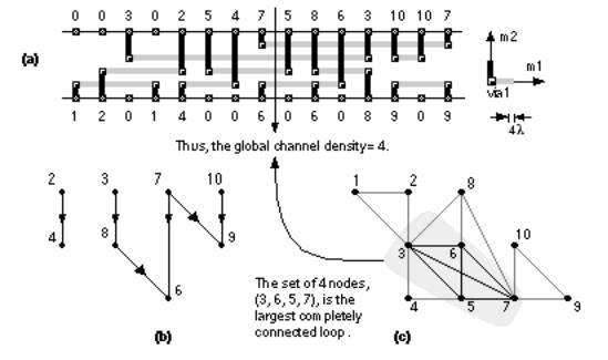
FIGURE 17.16 Routing graphs. (a) Channel with a global density of 4. (b) The vertical constraint graph. If two nets occupy the same column, the net at the top of the channel imposes a vertical constraint on the net at the bottom. For example, net 2 imposes a vertical constraint on net 4. Thus the interconnect for net 4 must use a track above net 2. (c) Horizontal-constraint graph. If the segments of two nets overlap, they are connected in the horizontal-constraint graph. This graph determines the global channel density.

We can also define a horizontal constraint and a corresponding horizontal-constraint graph . If the trunk for net 1 overlaps the trunk of net 2, then we say there is a horizontal constraint between net 1 and net 2. Unlike a vertical constraint, a horizontal constraint has no direction. Figure 17.16 (c) shows an example of a horizontal constraint graph and shows a group of 4 terminals (numbered 3, 5, 6, and 7) that must all overlap. Since this is the largest such group, the global channel density is 4.

If there are no vertical constraints at all in a channel, we can guarantee that the LEA will find the minimum number of routing tracks. The addition of vertical constraints transforms the restricted routing problem into an NP-complete problem. There is also an arrangement of vertical constraints that none of the algorithms based on the LEA can cope with. In Figure 17.17 (a) net 1 is above net 2 in the first column of the channel. Thus net 1 imposes a vertical constraint on net 2. Net 2 is above net 1 in the last column of the channel. Then net 2 also imposes a vertical constraint on net 1. It is impossible to route this arrangement using two routing layers with the restriction of using only one trunk for each net. If we construct the vertical-constraint graph for this situation, shown in

Figure 17.17 (b), there is a loop or cycle between nets 1 and 2. If there is any such vertical-constraint cycle (or cyclic constraint ) between two or more nets, the LEA will fail. A dogleg router removes the restriction that each net can use only one track or trunk. Figure 17.17 (c) shows how adding a dogleg permits a

channel with a cyclic constraint to be routed.

FIGURE 17.17 The addition of a dogleg, an extra trunk, in the wiring of a net can resolve cyclic vertical constraints.

The channel-routing algorithms we have described so far do not allow interconnects on one layer to run on top of other interconnects on a different layer. These algorithms allow interconnects to cross at right angles to each other on different layers, but not to overlap . When we remove the restriction that horizontal and vertical routing must use different layers, the density of a channel is no longer the lower bound for the number of tracks required. For two routing layers the ultimate lower bound becomes half of the channel density. The practical reasoning for restricting overlap is the parasitic overlap capacitance between signal interconnects. As the dimensions of the metal interconnect are reduced, the capacitance between adjacent interconnects on the same layer ( coupling capacitance ) is comparable to the capacitance of interconnects that overlap on different layers ( overlap capacitance ). Thus, allowing a short overlap between interconnects on different layers may not be as bad as allowing two interconnects to run adjacent to each other for a long distance on the same layer. Some routers allow you to specify that two interconnects must not run adjacent to each other for more than a specified length.

The channel height is fixed for channeled gate arrays; it is variable in discrete steps for channelless gate arrays; it is continuously variable for cell-based ASICs. However, for all these types of ASICs, the channel wiring is fully customized and so may be compacted or compressed after a channel router has completed the interconnect. The use of channel-routing compaction for a two-layer channel can reduce the channel height by 15 percent to 20 percent [ Cheng et al., 1992].

Modern channel routers are capable of routing a channel at or near the theoretical minimum density. We can thus consider channel routing a solved problem. Most of the difficulty in detailed routing now comes from the need to route more than two layers and to route arbitrary shaped regions. These problems are best handled by area routers.

17.2.6 Area-Routing Algorithms

There are many algorithms used for the detailed routing of general-shaped areas (see the paper by Ohtsuki in [ Ohtsuki, 1986]). Many of these were originally developed for PCB wiring. The first group we shall cover and the earliest to be used historically are the grid-expansion or maze-running algorithms. A second group of methods, which are more efficient, are the line-search algorithms.

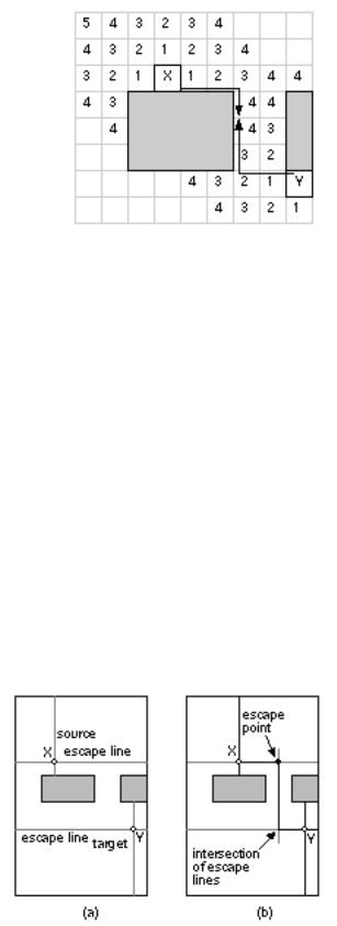
FIGURE 17.18 The Lee maze-running algorithm. The algorithm finds a path from source (X) to target (Y) by emitting a wave from both the source and the target at the same time. Successive outward moves are marked in each bin. Once the target is reached, the path is found by backtracking (if there is a choice of bins with equal labeled values, we choose the bin that avoids changing direction). (The original form of the Lee algorithm uses a single wave.)

Figure 17.18 illustrates the Lee maze-running algorithm . The goal is to find a path from X to Y i.e., from the start (or source) to the finish (or target) avoiding any obstacles. The algorithm is often called wave propagation because it sends out waves, which spread out like those created by dropping a stone into a pond.

Algorithms that use lines rather than waves to search for connections are more efficient than algorithms based on the Lee algorithm. Figure 17.19 illustrates the Hightower algorithm a line-search algorithm (or line-probe algorithm ):

1.Extend lines from both the source and target toward each other.

2.When an extended line, known as an escape line , meets an obstacle, choose a point on the escape line from which to project another escape line at right angles to the old one. This point is the escape point .

3.Place an escape point on the line so that the next escape line just misses the edge of the obstacle. Escape lines emanating from the source and target intersect to form the path.

FIGURE 17.19 Hightower area-routing algorithm. (a) Escape lines are constructed from source (X) and target (Y) toward each other until they hit obstacles. (b) An escape point is found on the escape line so that the next escape line perpendicular to the original misses the next obstacle. The path is complete when escape lines from source and target meet.

The Hightower algorithm is faster and requires less memory than methods based on the Lee algorithm.

17.2.7 Multilevel Routing

Using two-layer routing , if the logic cells do not contain any m2, it is possible to complete some routing in m2 using over-the-cell (OTC) routing. Sometimes poly is used for short connections in the channel in a two-level metal technology; this is known as 2.5-layer routing . Using a third level of metal in three-layer routing , there is a choice of approaches. Reserved-layer routing restricts all the interconnect on each layer to flow in one direction in a given routing area (for example, in a channel, either parallel or perpendicular to the channel spine). Unreserved-layer routing moves in both horizontal and vertical directions on a given layer. Most routers use reserved routing. Reserved three-level metal routing offers another choice: Either use m1 and m3 for horizontal routing (parallel to the channel spine), with m2 for vertical routing ( HVH routing ) or use VHV routing

. Since the logic cell interconnect usually blocks most of the area on the m1 layer, HVH routing is normally used. It is also important to consider the pitch of the layers when routing in the same direction on two different layers. Using HVH routing it is preferable for the m3 pitch to be a simple multiple of the m1 pitch (ideally they are the same). Some processes have more than three levels of metal. Sometimes the upper one or two metal layers have a coarser pitch than the lower layers and are used in multilevel routing for power and clock lines rather than for signal interconnect.

Figure 17.20 shows an example of three-layer channel routing. The logic cells are 64 l high, the m1 routing pitch is 8 l, and the m2 and m3 routing pitch is 16 l . The channel in Figure 17.20 is the same as the channel using two-layer metal shown in Figure 17.13 , but using three-level metal reduces the channel height from 40 l ( = 5 ¥ 8 l ) to 16 l . Submicron processes try to use the same metal pitch on all metal layers. This makes routing easier but processing more difficult.

FIGURE 17.20 Three-level channel routing. In this diagram the m2 and m3 routing pitch is set to twice the m1 routing pitch. Routing density can be increased further if all the routing pitches can be made equal a difficult process challenge.

With three or more levels of metal routing it is possible to reduce the channel height in a row-based ASIC to zero. All of the interconnect is then completed over the cell. If all of the channels are eliminated, the core area (logic cells plus routing) is determined solely by the logic-cell area. The point at which this happens depends on not only the number of metal layers and channel density, but also the routing resources (the blockages and feedthroughs) in the logic cell. This the cell porosity . Designing porous cells that help to minimize routing area is an art. For example, it is quite common to be able to produce a smaller chip using larger logic cells if the larger cells have more routing resources.

17.2.8 Timing-Driven Detailed Routing

In detailed routing the global router has already set the path the interconnect will follow. At this point little can be done to improve timing except to reduce the number of vias, alter the interconnect width to optimize delay, and minimize overlap capacitance. The gains here are relatively small, but for very long branching nets even small gains may be important. For high-frequency clock nets it may be important to shape and chamfer (round) the interconnect to match impedances at branches and control reflections at corners.

17.2.9 Final Routing Steps

If the algorithms to estimate congestion in the floorplanning tool accurately perfectly reflected the algorithms used by the global router and detailed router, routing completion should be guaranteed. Often, however, the detailed router will not be able to completely route all the nets. These problematical nets are known as unroutes . Routers handle this situation in one of two ways. The first method leaves the problematical nets unconnected. The second method completes all interconnects anyway but with some design-rule violations (the problematical nets may be shorted to other nets, for example). Some tools flag these problems as a warning (in fact there can be no more serious error).

If there are many unroutes the designer needs to discover the reason and return to the floorplanner and change channel sizes (for a cell-based ASIC) or increase the base-array size (for a gate array). Returning to the global router and changing bin sizes or adjusting the algorithms may also help. In drastic cases it may be necessary to change the floorplan. If just a handful of difficult nets remain to be routed, some tools allow the designer to perform hand edits using a rip-up and reroute router (sometimes this is done automatically by the detailed router as a last phase in the routing procedure anyway). This capability also permits

engineering change orders ( ECO ) corresponding to the little yellow wires on a PCB. One of the last steps in routing is via removal the detailed router looks to see if it can eliminate any vias (which can contribute a significant amount to the interconnect resistance) by changing layers or making other modifications to the completed routing. Routing compaction can then be performed as the final step.