15.7 Partitioning Methods

System partitioning requires goals and objectives, methods and algorithms to find solutions, and ways to evaluate these solutions. We start with measuring connectivity, proceed to an example that illustrates the concepts of system partitioning and then to the algorithms for partitioning.

Assume that we have decided which parts of the system will use ASICs. The goal of partitioning is to divide this part of the system so that each partition is a single ASIC. To do this we may need to take into account any or all of the following objectives:

●A maximum size for each ASIC

●A maximum number of ASICs

●A maximum number of connections for each ASIC

●A maximum number of total connections between all ASICs

We know how to measure the first two objectives. Next we shall explain ways to measure the last two.

15.7.1 Measuring Connectivity

To measure connectivity we need some help from the mathematics of graph theory. It turns out that the terms, definitions, and ideas of graph theory are central to ASIC construction, and they are often used in manuals and books that describe the knobs and dials of ASIC design tools.

FIGURE 15.6 Networks, graphs, and partitioning. (a) A network containing circuit logic cells and nets. (b) The equivalent graph with vertexes and edges. For example: logic cell D maps to node D in the graph; net 1 maps to the edge (A, B) in the graph. Net 3 (with three connections) maps to three edges in the graph: (B, C), (B, F), and (C, F). (c) Partitioning a network and its graph. A network with a net cut that cuts two nets. (d) The network graph showing the corresponding edge cut. The net cutset in c contains two nets, but the corresponding edge cutset in d contains four edges. This means a graph is not an exact model of a network for partitioning purposes.

Figure 15.6 (a) shows a circuit schematic, netlist, or network. The network consists of circuit modules A F. Equivalent terms for a circuit module are a cell, logic cell, macro, or a block. A cell or logic cell usually refers to a small logic gate (NAND etc.), but can also be a collection of other cells; macro refers to gate-array cells; a block is usually a collection of gates or cells. We shall use the term logic cell in this chapter to cover all of these.

Each logic cell has electrical connections between the terminals ( connectors or pins). The network can be represented as the mathematical graph shown in Figure 15.6 (b). A graph is like a spider s web: it contains vertexes (or vertices) AF (also known as graph nodes or points) that are connected by edges. A graph vertex corresponds to a logic cell. An electrical connection (a net or a signal) between two logic cells corresponds to a graph edge.

Figure 15.6 (c) shows a network with nine logic cells A I. A connection, for

example between logic cells A and B in Figure 15.6 (c), is written as net (A, B). Net (A, B) is represented by the single edge (A, B) in the network graph, shown in Figure 15.6 (d). A net with three terminals, for example net (B, C, F), must be modeled with three edges in the network graph: edges (B, C), (B, F), and (C, F). A net with four terminals requires six edges and so on. Figure 15.6 illustrates the differences between the nets of a network and the edges in the network graphs.

Notice that a net can have more than two terminals, but a terminal has only one net.

If we divide, or partition, the network shown in Figure 15.6 (c) into two parts, corresponding to creating two ASICs, we can divide the network s graph in the same way. Figure 15.6 (d) shows a possible division, called a cutset. We say that there is a net cutset (for the network) and an edge cutset (for the graph). The connections between the two ASICs are external connections, the connections inside each ASIC are internal connections.

Notice that the number of external connections is not modeled correctly by the network graph. When we divide the network into two by drawing a line across connections, we make net cuts. The resulting set of net cuts is the net cutset. The number of net cuts we make corresponds to the number of external connections between the two partitions. When we divide the network graph into the same partitions we make edge cuts and we create the edge cutset. We have already shown that nets and graph edges are not equivalent when a net has more than two terminals. Thus the number of edge cuts made when we partition a graph into two is not necessarily equal to the number of net cuts in the network. As we shall see presently the differences between nets and graph edges is important when we consider partitioning a network by partitioning its graph [ Schweikert and Kernighan, 1979].

15.7.2 A Simple Partitioning Example

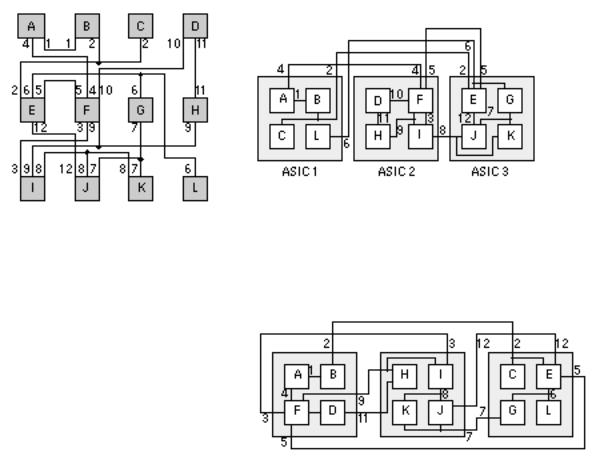
Figure 15.7 (a) shows a simple network we need to partition [ Goto and Matsud, 1986]. There are 12 logic cells, labeled A L, connected by 12 nets (labeled 1 12). At this level, each logic cell is a large circuit block and might be RAM, ROM, an ALU, and so on. Each net might also be a bus, but, for the moment, we assume that each net is a single connection and all nets are weighted equally. The goal is to partition our simple network into ASICs. Our objectives are the following:

●Use no more than three ASICs.

●Each ASIC is to contain no more than four logic cells.

●Use the minimum number of external connections for each ASIC.

●Use the minimum total number of external connections.

Figure 15.7 (b) shows a partitioning with five external connections; two of the ASICs have three pins; the third has four pins.We might be able to find this arrangement by hand, but for larger systems we need help.

(a)

(b)

FIGURE 15.7 Partitioning example. (a) We wish to partition this network into three

ASICs with no more than four (c) logic cells per ASIC. (b) A partitioning with five external connections (nets 2, 4, 5, 6, and 8) the minimum number. (c) A constructed partition using

logic cell C as a seed. It is difficult to get from this local minimum, with seven external connections (2, 3, 5, 7, 9,11,12), to the optimum solution of b.

Splitting a network into several pieces is a network partitioning problem. In the following sections we shall examine two types of algorithms to solve this problem and describe how they are used in system partitioning. Section 15.7.3 describes constructive partitioning, which uses a set of rules to find a solution. Section 15.7.4 describes iterative partitioning improvement (or iterative partitioning refinement), which takes an existing solution and tries to improve it. Often we apply iterative improvement to a constructive partitioning. We also use many of these partitioning algorithms in solving floorplanning and placement problems that we shall discuss in Chapter 16.

15.7.3 Constructive Partitioning

The most common constructive partitioning algorithms use seed growth or cluster growth. A simple seed-growth algorithm for constructive partitioning consists of the following steps:

1.Start a new partition with a seed logic cell.

2.Consider all the logic cells that are not yet in a partition. Select each of

these logic cells in turn.

3.Calculate a gain function, g(m) , that measures the benefit of adding logic cell m to the current partition. One measure of gain is the number of connections between logic cell m and the current partition.

4.Add the logic cell with the highest gain g(m) to the current partition.

5.Repeat the process from step 2. If you reach the limit of logic cells in a partition, start again at step 1.

We may choose different gain functions according to our objectives (but we have to be careful to distinguish between connections and nets). The algorithm starts with the choice of a seed logic cell ( seed module, or just seed). The logic cell with the most nets is a good choice as the seed logic cell. You can also use a set of seed logic cells known as a cluster. Some people also use the term cliqueborrowed from graph theory. A clique of a graph is a subset of nodes where each pair of nodes is connected by an edge like your group of friends at school where everyone knows everyone else in your clique . In some tools you can use schematic pages (at the leaf or lowest hierarchical level) as a starting point for partitioning. If you use a high-level design language, you can use a Verilog module (different from a circuit module) or VHDL entity/architecture as seeds (again at the leaf level).

15.7.4 Iterative Partitioning

Improvement

The most common iterative improvement algorithms are based on interchange and group migration. The process of interchanging (swapping) logic cells in an effort to improve the partition is an interchange method. If the swap improves the partition, we accept the trial interchange; otherwise we select a new set of logic cells to swap.

There is a limit to what we can achieve with a partitioning algorithm based on simple interchange. For example, Figure 15.7 (c) shows a partitioning of the network of part a using a constructed partitioning algorithm with logic cell C as the seed. To get from the solution shown in part c to the solution of part b, which has a minimum number of external connections, requires a complicated swap. The three pairs: D and F, J and K, C and L need to be swapped all at the same time. It would take a very long time to consider all possible swaps of this complexity. A simple interchange algorithm considers only one change and rejects it immediately if it is not an improvement. Algorithms of this type are greedy algorithms in the sense that they will accept a move only if it provides immediate benefit. Such shortsightedness leads an algorithm to a local minimum from which it cannot escape. Stuck in a valley, a greedy algorithm is not prepared to walk over a hill to see if there is a better solution in the next valley. This type of problem occurs repeatedly in CAD algorithms.

Group migration consists of swapping groups of logic cells between partitions. The group migration algorithms are better than simple interchange methods at improving a solution but are more complex. Almost all group migration methods are based on the powerful and general Kernighan Lin algorithm ( K L algorithm) that partitions a graph [ Kernighan and Lin, 1970]. The problem of dividing a graph into two pieces, minimizing the nets that are cut, is the min-cut problem a very important one in VLSI design. As the next section shows, the K L algorithm can be applied to many different problems in ASIC design. We shall examine the algorithm next and then see how to apply it to system partitioning.

15.7.5 The Kernighan Lin Algorithm

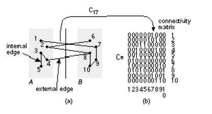
Figure 15.8 illustrates some of the terms and definitions needed to describe the KL algorithm. External edges cross between partitions; internal edges are contained inside a partition. Consider a network with 2 m nodes (where m is an integer) each of equal size. If we assign a cost to each edge of the network graph, we can define a cost matrix C = c ij , where c ij = c ji and c ii = 0. If all connections are equal in importance, the elements of the cost matrix are 1 or 0, and in this special case we usually call the matrix the connectivity matrix. Costs higher than 1 could represent the number of wires in a bus, multiple connections to a single logic cell, or nets that we need to keep close for timing reasons.

FIGURE 15.8 Terms used by the Kernighan Lin partitioning algorithm. (a) An example network graph. (b) The connectivity matrix, C; the column and rows are labeled to help you see how the matrix entries correspond to the node numbers in the graph. For example, C 17 (column 1, row 7) equals 1 because nodes 1 and 7 are connected. In this example all edges have an equal weight of 1, but in general the edges may have different weights.

Suppose we already have split a network into two partitions, A and B , each with m nodes (perhaps using a constructed partitioning). Our goal now is to swap nodes between A and B with the objective of minimizing the number of external edges connecting the two partitions. Each external edge may be weighted by a cost, and our objective corresponds to minimizing a cost function that we shall

call the total external cost, cut cost, or cut weight, W :

a A , b B

In Figure 15.8 (a) the cut weight is 4 (all the edges have weights of 1).

In order to simplify the measurement of the change in cut weight when we interchange nodes, we need some more definitions. First, for any node a in partition A , we define an external edge cost, which measures the connections from node a to B ,

For example, in Figure 15.8 (a) E 1 = 1, and E 3 = 0. Second, we define the internal edge cost to measure the internal connections to a ,

.(15.2)

So, in Figure 15.8 (a), I 1 = 0, and I 3 = 2. We define the edge costs for partition B in a similar way (so E 8 = 2, and I 8 = 1). The cost difference is the difference between external edge costs and internal edge costs,

D x = E x I x . (15.16)

Thus, in Figure 15.8 (a) D 1 = 1, D 3 = 2, and D 8 = 1. Now pick any node in A , and any node in B . If we swap these nodes, a and b, we need to measure the reduction in cut weight, which we call the gain, g . We can express g in terms of the edge costs as follows:

g = D a + D b 2 c ab . (15.17)

The last term accounts for the fact that a and b may be connected. So, in Figure 15.8 (a), if we swap nodes 1 and 6, then g = D 1 + D 6 2 c 16 = 1 + 1. If we swap nodes 2 and 8, then g = D 2 + D 8 2 c 28 = 1 + 2 2.

The K L algorithm finds a group of node pairs to swap that increases the gain even though swapping individual node pairs from that group might decrease the gain. First we pretend to swap all of the nodes a pair at a time. Pretend swaps are like studying chess games when you make a series of trial moves in your head.

This is the algorithm:

1. Find two nodes, a i from A , and b i from B , so that the gain from

swapping them is a maximum. The gain is

gi = D ai + D bi 2 c aibi . (15.18)

2.Next pretend swap a i and b i even if the gain g i is zero or negative, and do not consider a i and b i eligible for being swapped again.

3.Repeat steps 1 and 2 a total of m times until all the nodes of A and B have been pretend swapped. We are back where we started, but we have ordered pairs of nodes in A and B according to the gain from interchanging those pairs.

4.Now we can choose which nodes we shall actually swap. Suppose we only swap the first n pairs of nodes that we found in the preceding process. In other words we swap nodes X = a 1 , a 2 ,&, a n from A with nodes Y = b 1 , b 2 ,&, b n from B. The total gain would be

n

G n = S g i . (15.19) i = 1

5. We now choose n corresponding to the maximum value of G n .

If the maximum value of G n > 0, then we swap the sets of nodes X and Y and thus reduce the cut weight by G n . We use this new partitioning to start the process again at the first step. If the maximum value of G n = 0, then we cannot improve the current partitioning and we stop. We have found a locally optimum solution.

Figure 15.9 shows an example of partitioning a graph using the K L algorithm. Each completion of steps 1 through 5 is a pass through the algorithm. Kernighan and Lin found that typically 2 4 passes were required to reach a solution. The most important feature of the K L algorithm is that we are prepared to consider moves even though they seem to make things worse. This is like unraveling a tangled ball of string or solving a Rubik s cube puzzle. Sometimes you need to make things worse so they can get better later. The K L algorithm works well for partitioning graphs. However, there are the following problems that we need to address before we can apply the algorithm to network partitioning:

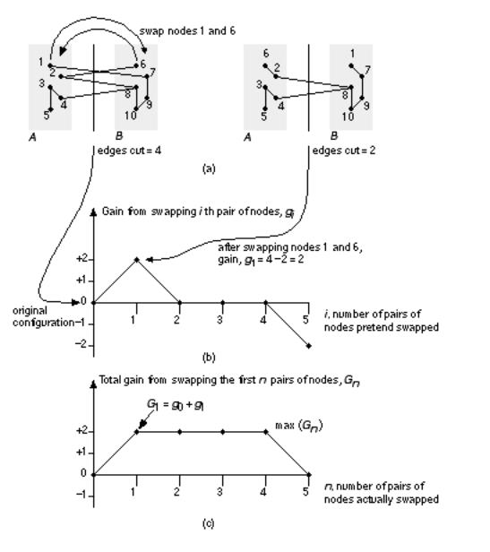
FIGURE 15.9 Partitioning a graph using the Kernighan Lin algorithm.

(a) Shows how swapping node 1 of partition A with node 6 of partition B results in a gain of g = 1. (b) A graph of the gain resulting from swapping pairs of nodes. (c) The total gain is equal to the sum of the gains obtained at each step.

●It minimizes the number of edges cut, not the number of nets cut.

●It does not allow logic cells to be different sizes.

●It is expensive in computation time.

●It does not allow partitions to be unequal or find the optimum partition size.

●It does not allow for selected logic cells to be fixed in place.

●The results are random.

●It does not directly allow for more than two partitions.

To implement a net-cut partitioning rather than an edge-cut partitioning, we can

just keep track of the nets rather than the edges [ Schweikert and Kernighan, 1979]. We can no longer use a connectivity or cost matrix to represent connections, though. Fortunately, several people have found efficient data structures to handle the bookkeeping tasks. One example is the FiducciaMattheyses algorithm to be described shortly.

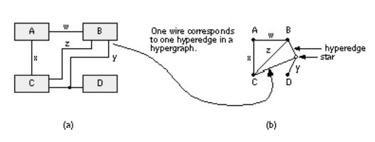
To represent nets with multiple terminals in a network accurately, we can extend the definition of a network graph. Figure 15.10 shows how a hypergraph with a special type of vertex, a star, and a hyperedge, represents a net with more than two terminals in a network.

FIGURE 15.10 A hypergraph. (a) The network contains a net y with three terminals. (b) In the network hypergraph we can model net y by a single hyperedge (B, C, D) and a star node. Now there is a direct correspondence between wires or nets in the network and hyperedges in the graph.

In the K L algorithm, the internal and external edge costs have to be calculated for all the nodes before we can select the nodes to be swapped. Then we have to find the pair of nodes that give the largest gain when swapped. This requires an amount of computer time that grows as n 2 log n for a graph with 2n nodes. This n 2 dependency is a major problem for partitioning large networks. The FiducciaMattheyses algorithm (the F M algorithm) is an extension to the K L algorithm that addresses the differences between nets and edges and also reduces the computational effort [ Fiduccia and Mattheyses, 1982]. The key features of this algorithm are the following:

●Only one logic cell, the base logic cell, moves at a time. In order to stop the algorithm from moving all the logic cells to one large partition, the base logic cell is chosen to maintain balance between partitions. The balance is the ratio of total logic cell size in one partition to the total logic cell size in the other. Altering the balance allows us to vary the sizes of the partitions.

●Critical nets are used to simplify the gain calculations. A net is a critical net if it has an attached logic cell that, when swapped, changes the number of nets cut. It is only necessary to recalculate the gains of logic cells on critical nets that are attached to the base logic cell.

●The logic cells that are free to move are stored in a doubly linked list. The lists are sorted according to gain. This allows the logic cells with maximum gain to be found quickly.

These techniques reduce the computation time so that it increases only slightly more than linearly with the number of logic cells in the network, a very important improvement [Fiduccia and Mattheyses, 1982].

Kernighan and Lin suggested simulating logic cells of different sizes by clumping s logic cells together with highly weighted nets to simulate a logic cell of size s . The F M algorithm takes logic-cell size into account as it selects a logic cell to swap based on maintaining the balance between the total logic-cell size of each of the partitions. To generate unequal partitions using the K L algorithm, we can introduce dummy logic cells with no connections into one of the partitions. The F M algorithm adjusts the partition size according to the balance parameter.

Often we need to fix logic cells in place during partitioning. This may be because we need to keep logic cells together or apart for reasons other than connectivity, perhaps due to timing, power, or noise constraints. Another reason to fix logic cells would be to improve a partitioning that you have already partially completed. The F M algorithm allows you to fix logic cells by removing them from consideration as the base logic cells you move. Methods based on the K L algorithm find locally optimum solutions in a random fashion. There are two reasons for this. The first reason is the random starting partition. The second reason is that the choice of nodes to swap is based on the gain. The choice between moves that have equal gain is arbitrary. Extensions to the K L algorithm address both of these problems. Finding nodes that are naturally grouped or clustered and assigning them to one of the initial partitions improves the results of the K L algorithm. Although these are constructive partitioning methods, they are covered here because they are closely linked with the K L iterative improvement algorithm.

15.7.6 The Ratio-Cut Algorithm

The ratio-cut algorithm removes the restriction of constant partition sizes. The cut weight W for a cut that divides a network into two partitions, A and B , is given by

W = S c ab

The K L algorithm minimizes W while keeping partitions A and B the same size. The ratio of a cut is defined as

W

R = (15.21) | A | | B |

In this equation | A | and | B | are the sizes of partitions A and B . The size of a partition is equal to the number of nodes it contains (also known as the set cardinality). The cut that minimizes R is called the ratio cut. The original description of the ratio-cut algorithm uses ratio cuts to partition a network into small, highly connected groups. Then you form a reduced network from these groups each small group of logic cells forms a node in the reduced network. Finally, you use the F M algorithm to improve the reduced network [ Cheng and Wei, 1991].

15.7.7 The Look-ahead Algorithm

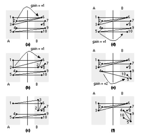
Both the K L and F M algorithms consider only the immediate gain to be made by moving a node. When there is a tie between nodes with equal gain (as often happens), there is no mechanism to make the best choice. This is like playing chess looking only one move ahead. Figure 15.11 shows an example of two nodes that have equal gains, but moving one of the nodes will allow a move that has a higher gain later.

FIGURE 15.11 An example of network partitioning that shows the need to look ahead when selecting logic cells to be moved between partitions. Partitionings (a), (b), and (c) show one sequence of moves, partitionings (d), (e), and (f) show a second sequence. The partitioning in (a) can be improved by moving node 2 from A to B with a gain of 1. The result of this move is shown in (b). This partitioning can be improved by moving node 3 to B, again with a gain of 1. The partitioning shown in (d) is the same as (a). We can move node 5 to B with a gain of 1 as shown in (e), but now we can move node 4 to B with a gain of 2.

We call the gain for the initial move the first-level gain. Gains from subsequent moves are then second-level and higher gains. We can define a gain vector that contains these gains. Figure 15.11 shows how the first-level and second-level gains are calculated. Using the gain vector allows us to use a look-ahead algorithm in the choice of nodes to be swapped. This reduces both the mean and variation in the number of cuts in the resulting partitions.

We have described algorithms that are efficient at dividing a network into two pieces. Normally we wish to divide a system into more than two pieces. We can do this by recursively applying the algorithms. For example, if we wish to divide a system network into three pieces, we could apply the F M algorithm first, using a balance of 2:1, to generate two partitions, with one twice as large as the other. Then we apply the algorithm again to the larger of the two partitions, with a balance of 1:1, which will give us three partitions of roughly the same size.

15.7.8 Simulated Annealing

A different approach to solving large graph problems (and other types of problems) that arise in VLSI layout, including system partitioning, uses the simulated-annealing algorithm [ Kirkpatrick et al., 1983]. Simulated annealing takes an existing solution and then makes successive changes in a series of random moves. Each move is accepted or rejected based on an energy function, calculated for each new trial configuration. The minimums of the energy function correspond to possible solutions. The best solution is the global minimum.

So far the description of simulated annealing is similar to the interchange algorithms, but there is an important difference. In an interchange strategy we accept the new trial configuration only if the energy function decreases, which means the new configuration is an improvement. However, in the simulated-annealing algorithm, we accept the new configuration even if the energy function increases for the new configuration which means things are getting worse. The probability of accepting a worse configuration is controlled by the exponential expression exp( D E / T ), where D E is the resulting increase in the energy function. The parameter T is a variable that we control and corresponds to the temperature in the annealing of a metal cooling (this is why the process is called simulated annealing).

We accept moves that seemingly take us away from a desirable solution to allow the system to escape from a local minimum and find other, better, solutions. The name for this strategy is hill climbing. As the temperature is slowly decreased, we decrease the probability of making moves that increase the energy function. Finally, as the temperature approaches zero, we refuse to make any moves that increase the energy of the system and the system falls and comes to rest at the nearest local minimum. Hopefully, the solution that corresponds to the minimum we have found is a good one.

The critical parameter governing the behavior of the simulated-annealing algorithm is the rate at which the temperature T is reduced. This rate is known as the cooling schedule. Often we set a parameter a that relates the temperatures, T i and T i + 1 , at the i th and i + 1th iteration:

T i +1 = a T i . (15.22)

To find a good solution, a local minimum close to the global minimum, requires a high initial temperature and a slow cooling schedule. This results in many trial moves and very long computer run times [ Rose, Klebsch, and Wolf, 1990]. If we are prepared to wait a long time (forever in the worst case), simulated annealing is useful because we can guarantee that we can find the optimum solution. Simulated annealing is useful in several of the ASIC construction steps and we shall return to it in Section 16.2.7.

15.7.9 Other Partitioning Objectives

In partitioning a real system we need to weight each logic cell according to its area in order to control the total areas of each ASIC. This can be done if the area of each logic cell can either be calculated or estimated. This is usually done as part of floorplanning, so we may need to return to partitioning after floorplanning.

There will be many objectives or constraints that we need to take into account during partitioning. For example, certain logic cells in a system may need to be located on the same ASIC in order to avoid adding the delay of any external interconnections. These timing constraints can be implemented by adding weights to nets to make them more important than others. Some logic cells may consume more power than others and you may need to add power constraints to avoid exceeding the power-handling capability of a single ASIC. It is difficult, though, to assign more than rough estimates of power consumption for each logic cell at the system planning stage, before any simulation has been completed. Certain logic cells may only be available in a certain technology if you want to include memory on an ASIC, for example. In this case, technology constraints will keep together logic cells requiring similar technologies. We probably want to impose cost constraints to implement certain logic cells in the lowest cost technology available or to keep ASICs below a certain size in order to use a

low-cost package. The type of test strategy you adopt will also affect the partitioning of logic. Large RAM blocks may require BIST circuitry; large amounts of sequential logic may require scan testing, possibly with a boundary-scan interface. One of the objects of testability is to maintain controllability and observability of logic inside each ASIC. In order to do this, test constraints may require that we force certain connections to be external. No automated partitioning tools can take into account all of these constraints. The best CAD tool to help you with these decisions is a spreadsheet.