Distance Separation plot under the Multi-Base Plots provides a good graphic to choose a proper tolerance.

2.Use low PPM values. Try either using the Very Low setting under Distance effect amount or even manually setting the horizontal PPM to 0.05 or as low as 0.02.

The first method is far more preferable.

9.6.11How can I speed up processing?

MB-KF processing can be much slower due to the increased numbers of states and observations. For example, 12 satellites on 4 bases will result in 50 states and 132 observations on every epoch. Therefore, here are some tips to cut down processing time without buying a faster computer:

•Disable any bases that are far outside of the project area, as they will add very little to final accuracies and may even hinder them.

•Consider disabling the Doppler measurement from processing. This is performed from Settings |

Individual | Advanced. Under Velocity/Doppler, disable Doppler measurement usage for phase processing. If accurate velocity is needed, enable it again in the final stage.

•Reduce the data interval for preliminary analysis to something like 2 seconds. One of the problems is that 1 or 2 Hz data can result in different effects and problems. This can be helped by forcing KAR to use the same data, which is accomplished under Settings | Individual | KAR. The processing value should be entered in the Search on data interval field. Be sure also to enable Only search on exact interval. This will help to make 2 second and high data rate data produce similar results, although it is best not to continue on this low data rate too long.

•Utilize only the closest base for fixed solutions. Consider lowering the maximum distance for fixed static usage under Settings | Individual | Advanced.

•Ensure that simultaneous forward and reverse processing is enabled for Xeon and dual CPU machines. See the Solution tab under Settings | Preferences.

•For projects with very large base separations, try limiting the maximum baseline distance. This can be set from the Measurement tab, which causes GrafNav to only use those bases which are within a certain distance. This increases speed and may improve accuracies.

9.7PPP (Precise Point Positioning)

9.7.1What is Precise Point Positioning?

Precise Point Positioning (PPP) is a form of GPS data post-processing that does not use a base station for differential corrections. It is performed using the observation data from one receiver, in conjunction with precise satellite orbit and clock files, which serve to minimize the error sources.

9.7.2How does PPP differ from differential processing?

The most obvious difference between PPP and differential processing is that a base station is not needed for PPP. Differential processing requires that a point with known coordinates be observed concurrently with the observations at an unknown point or remote trajectory. In PPP, only the observations associated with the unknown points are needed.

Differential processing relies on concurrent observations made to the same satellites from two different receivers to form a double-differencing equation that eliminates or reduces the major sources of error associated with GPS. Without the benefit of concurrent observations, PPP is left to deal with these errors sources in a different manner. For

example, the satellite clock errors (dt), which are removed through double-differencing in differential processing, are reduced in PPP through the use of a high-rate 30-second precise clock file. The same applies to the satellite orbit errors (dρ), which are essentially eliminated for shorter baselines in differential mode, but are instead reduced through the use of precise orbit files in PPP. These precise satellite clock and orbit files are generated by various agencies (IGS, JPL, GFZ, and others) using data collected by a worldwide network of receivers.

When processing differentially, the major component of the tropospheric error is removed through the differencing procedure, leaving only the relative error to be dealt with. In PPP, the absolute error must be accounted for, and this is done by modeling the tropospheric zenith delay as a state in the Kalman filter.

Also, whereas double-differencing only solves for three position components (X, Y, Z), PPP is left to solve for a fourth unknown, namely the receiver clock error (dT), which has not been differenced out.

The integer ambiguity values are not solved for in PPP, but are instead left to converge as floating point values. Although not always realized, differential processing does offer the potential to do so.

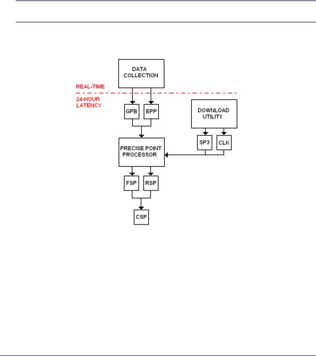
See Figure 7 on page 276 for a flow diagram of the PPP procedure.

Figure 7: PPP Procedure

9.7.3How accurate is PPP?

When carrier phase ambiguities are resolved, differential processing can offer centimeter-level accuracy, which would be unreasonable to expect from PPP. Testing has shown that, in the presence of good-quality, uninterrupted dual frequency phase measurements, the PPP can converge to accuracies of 10cm-30cm on kinematic data sets. For static data sets, the accuracies are largely dependent on the length of time that the point is observed. Test data sets have produced a final position within 1-2 cm horizontally and 2-3cm vertically of the truth coordinates when spanning 24 hours. Testing has also consistently produced coordinates within 2.5cm horizontally and 5cm vertically of the truth on 6 hour data sets, and 7cm horizontally and vertically on 2 hour data sets. It is very important to keep in mind here that the achieved accuracies will be dependent on many factors, ranging from satellite availability to receiver noise characteristics. The accuracies provided above are done so only as a guideline, and not as a guarantee.