

GrafNav |
Chapter 2 |
|
|
|
|
2.5 Process Menu
2.5.1Process GNSS (differential)
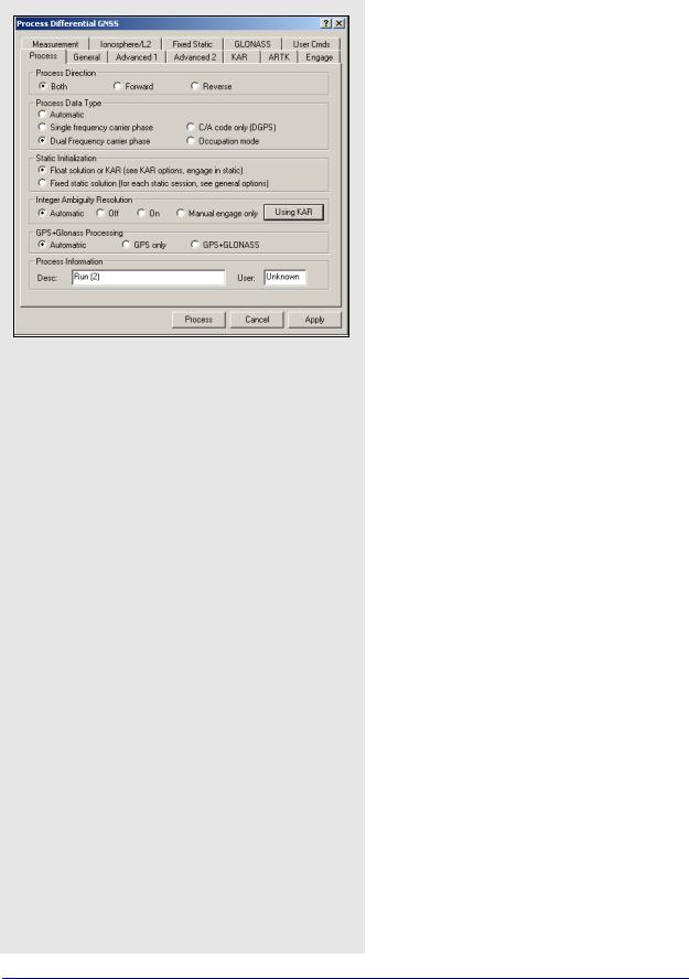
The Process GPS or GPS+GLONASS window provides access to most settings related to differential processing and lets you choose the options best suited to your application.
Process
Process Direction
Defines which time direction to process data in. The direction options are in the shaded box.
Process Data Type
Defines the type of data used for processing including the following:
Automatic
Detects dual frequency, single frequency or code only receiver data. If the master(s) and remote are logging different data types, then it selects the one with the least measurements.
The order of increasing measurement availability is C/A code only, single frequency, and then dual frequency. If L2 tracking is very poor, then a dual frequency GPS receiver may be detected as single frequency.
Single frequency carrier phase
Processes with C/A code, L1 carrier phase and L1 Doppler data in a combined Kalman filter, so each variable must be available. Single frequency is generally more accurate than C/A code only. Carrier phase ambiguities can be fixed but the process is less reliable than the dual frequency mode because you can’t make ionospheric corrections.
Dual frequency carrier phase
Processes same measurements as single frequency mode, but with the addition of L2 carrier phase. Processing dual frequency has two benefits that are listed in the shaded box. By combining the L1 and L2 carrier phase the widelane is formed. When used for Fixed Static (KAR), this technique is more reliable, solves on longer distances and requires less observation time. For example, KAR resolves in few minutes what could take up to 20 minutes in single frequency mode.
Process direction options
Forward: Processes the data chronologically from the beginning and in the same direction that it was collected in.
Reverse: Starts processing the data from the end to the beginning.
Both: Processes in both directions. If this option is activated, the two solutions are combined after processing. See Section 2.6.10, on Page 102 for help doing so. This method is most effective for kinematic processing. For static processing, only use the forward or reverse options.
Benefits of using the dual frequency carrier phase
The benefits of processing in dual frequency mode include the following:
•Better accuracy on baselines longer than 10 km when ionospheric corrections are enabled.
•Improves the reliability of integer ambiguity search techniques.
GrafNav / GrafNet 8.10 User Guide Rev 4 |
61 |
Chapter 2 |
GrafNav |
|
|
C/A code only (DGPS(Differential Global Positioning System))
Processes in an advanced differential correction mode and is performed on data with little or no carrier phase information. For kinematic data, the accuracy is the same as real-time differential or RTCM corrections. In static mode, the accuracy is higher due to the averaging effect.
Occupation mode
This special mode of operation is designed for areas of heavy tree cover. In this mode, you should remain stationary over each point of interest for 2 to 5 minutes. In this mode, carrier phase lock does not have to be maintained during travel between points. Since the carrier phase is used only for static data, you can achieve sub-metre accuracies in this terrain. GLONASS processing is also suggested to include additional satellites.
Static Initialization
The two options are the following:
Float solution or KAR
This setting is necessary for kinematic initialization. For static data, the float solution does not solve for integer ambiguities, so it is less accurate than the Fixed Static solution. These integers are often not solvable for baselines greater than 10 km in single frequency and up to 25 km in dual frequency. In these cases, the float solution is the best alternative. For dual frequency data, enable the ionospheric free correction mode.
Fixed static solution
Processes the carrier phase to get a static fixed integer solution. If the integers are correctly determined, this mode is the most accurate. For longer static baselines, an ionospheric correction is applied to the fixed solution. For single frequency 15 minutes is suggested. For dual frequency, only a few minutes will work. To lessen the likelihood of having to reobserve a point, extend the time. Time should be increased with baseline lengths for both single and dual frequency. See Section 2.4.7, on Page 57 for important information regarding the processing of static sessions.
62 |
GrafNav / GrafNet 8.10 User Guide Rev 4 |

GrafNav |
Chapter 2 |
|
|
|
|
Integer Ambiguity Resolution
Both ARTK and KAR compute integer ambiguities for both static and kinematic trajectories. KAR is best suited to airborne applications and takes quite some time to resolve. ARTK, on the other hand, resolves very quickly, which can be a big benefit for ground vehicle applications where there are only short periods of continuous data between obstructions. In addition, ARTK fixes often, which is beneficial for ground mapping and surveying applications, as it maximizes ambiguity determination accuracy. However, in airborne, it can cause unnecessary jumps or spikes in the trajectory, thereby increasing relative positioning error. To mitigate this, it is suggested that the On engage only level is used for the Criteria for accepting new fixes setting. See ARTK Options on
Page 74. For relatively stationary or slow moving platforms, ARTK can fix on longer distances than KAR. For airborne, ARTK and KAR perform about the same in terms of fix distance.
Generally, ARTK produces fewer incorrect fixes than KAR, but this can vary by data set. ARTK currently does not fix GLONASS satellites. KAR can use GLONASS but the advantage is often minimal. For LiDAR users requiring the highest level of accuracy, ARTK can be a valuable tool. The integer ambiguity processing options are listed in the shaded box.
GPS+GLONASS Processing
Applies only to data logged using GLONASSenabled receivers. The processing option settings are listed in the shaded box.
Process Information
Lets you enter processing information and then stores it in the processing history. The options of types of information are listed in the shaded box.
Integer Ambiguity Resolution processing option settings
Automatic
Enables KAR for dual frequency and disables it for single.
Off
Forces KAR to never engage.
On
Forces KAR to be enabled for single and dual frequencies.
Manual Engage Only
KAR only engages at your selected times. Define these times under the Engage tab. See Section , on Page 75 for help.
Using KAR/ARTK
This button toggles between the ARTK and KAR algorithms for integer ambiguity resolution.
GPS + Glonass processing option settings
Automatic
Enables the use of available GLONASS data.
GPS only
Disables GLONASS processing. This option is useful if GLONASS data causes problems.
GPS+GLONASS
Forces the use of available GLONASS data. Use this option if automatic detection fails.
Types of Process Information:
Desc
Enter a description of the run here. The program numbers the runs numerically.
User
Enter your name or initials.
See Section 2.5, on Page 61 for more process options.
GrafNav / GrafNet 8.10 User Guide Rev 4 |
63 |
Chapter 2 |
GrafNav |
|
|
Data Interval option settings
Normal
For kinematic and float static processing, the program automatically synchronizes both the master and remote data sets at the collection rate. With this option, you can specify the interval to process the data. Entering zero results in all epochs being processed.
Fixed Static
Use this interval for the fixed static solution. The recommended interval for fixed static is 15 seconds. Shorter intervals result in overly optimistic accuracy estimates because of high time correlation of carrier phase data over periods less than 15 seconds and does not improve accuracies.
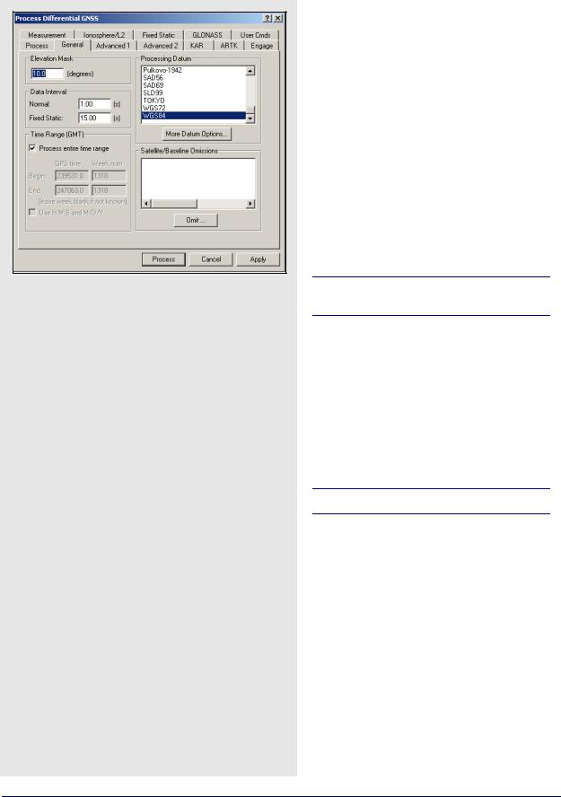
General
Elevation Mask
Defines the minimum elevation above the horizon that a satellite must reach before being used for processing. The default elevation cut-off is 10 degrees; 13 degrees has been found to work well for most airborne data sets.
You can raise the elevation to 15 degrees, but be aware that raising this value too high might cause satellites that are important to the geometry to be missed. Lowering this value is not suggested because it causes noisy satellites at low elevation to degrade the solution.
Data Interval
Defines the intervals to kinematic and static data at. The two setting options are described in the shaded box.
Data sets with only static data benefit from data intervals of 15 or 30 seconds.
Time Range
Defines the time range to be processed. If the
Process entire time range option is enabled, GrafNav processes starting at the first epoch the master and remote have in common and end at the last. To limit the scope of processing, use the Begin and End fields. The default time system is GPS seconds of the week (0-604800), but times can also be entered in hours, minutes and seconds if the Use H:M:S and M/D/Y option is selected.
Times are in GMT (Greenwhich mean time).
Processing Datum
By default, the processing datum is the same one that the base station coordinates are entered in. You have the option to process in a global datum and enter the coordinates in the local datum but this approach is more complex and should only be used if you thoroughly understand datums. Click on More Datum Options to do the following:
•to enable or disable datums
•to enable coordinate input in a datum different than the processing datum. See Section 2.6.5, on Page 97 for more information
64 |
GrafNav / GrafNet 8.10 User Guide Rev 4 |
GrafNav |
Chapter 2 |
|
|
|
|
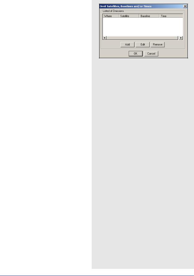
Omit Satellite Info
This option brings up the Omit Satellites, Baselines and/or Times window, in which you can enter omissions.
Satellites to Omit
All Satellites
Disables all satellites from being used.
Only specified satellite
Disables individual satellites.
Baselines to Omit
Omit satellite for all baselines
Applies the satellite omission to all baselines in the project.
Only selected baseline
Applies the satellite omission only to the specified baseline (applies to multi-baseline projects only).
Time Period
Omit for entire data set
Applies the omission to the entire processing time range.
Use specified time range
Applies the omission to a specific time period, entered in GPS seconds of the week.
Where to Omit
From processing
Applies the omission to all types of processing.
From KAR/Fixed-Static only
Applies the omission only during ambiguity resolution.
GrafNav / GrafNet 8.10 User Guide Rev 4 |
65 |
Chapter 2 |
GrafNav |
|
|
Dynamic/Velocity model settings
Automatic
This setting is suggested because it turns off dynamic constraint if Doppler measurement usage is enabled, and turns on High dynamic constraint setting if it is disabled.
High
Vehicle dynamics (100 m position error due to velocity change).
Med
Vehicle dynamics (10 m position error due to velocity change).
Low
Vehicle dynamics (1 m position error due to velocity change).
Off
No constraint.
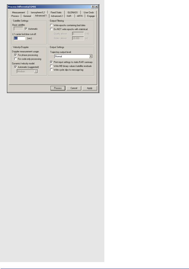
Advanced 1 Options
Satellite Settings
The two settings available here include the following:
Base satellite
Specifies the satellite to be initially used as the base for the differenced observations. Generally, Automatic selection is much preferred.
L1 carrier locktime cut-off:
The number of seconds of continuous carrier phase lock before data for that channel is deemed usable. This allows you to reject data for the first n seconds after acquiring lock. The default value is 4, but higher numbers (8 to 12 s) can be very beneficial to some GPS receivers, especially low-cost ones.
Velocity/Doppler
The following settings apply to the use of Doppler measurements.
Doppler measurement usage
The Doppler is mainly used for velocity determination. The default setting is For phase processing but you can disable it if several Doppler error warnings are present in the message log.
Dynamic/Velocity model
This setting controls when to use the constant velocity vehicle dynamic constraint. The main purpose of this setting is to improve velocity determination accuracy if the Doppler measurement usage is disabled. The settings available for this option are in the shaded box.
66 |
GrafNav / GrafNet 8.10 User Guide Rev 4 |

GrafNav |
Chapter 2 |
|
|
|
|
Output Filtering
This option has the two following settings that affect GrafNav’s handling of bad data:
Write epochs containing bad data
Prints out all positions that GrafNav computes, good or bad. GrafNav does not print positions for epochs where the Kalman filter detects large measurement errors. This option should only be used if you need a position for as many epochs as possible and if you are not concerned about various low quality positions.
Do not write epochs with poor statistics
This setting removes epochs from a solution that have quality numbers or standard deviations greater than the specified threshold. Use this option to try to filter out bad positions from the output.
Output Settings
These options pertain to the amount of information written to disk.
Trajectory output level
This option allows you to select the format of the epoch output files. The setting options in the drop-down menu are described in the shaded box.
Print input settings to static/KAR summary
Prints processing settings at the start of the FSS and RSS files. This is useful for recording the options that were used to create a solution file. After each run, a copy of the CFG file is also saved in the Process History.
Write MB binary values/satellite residuals
Writes carrier code and residuals for each satellite and baseline to FBV and RBV files. This setting are always enabled for MB processing.
Write cycle slips to message log
Prints satellite cycle slips and rising/falling messages to the FML and RML files. Disabling this option creates a more concise message log but these multiple messages might help locate a problem satellite.
Trajectory output level setting options
Normal
Default for GrafNav.
Extended (covariance)
This format is suggested for users who require additional information. It is identical to Normal except that additional fields exist for the relative vector information, position and velocity covariances, as well as the ambiguity values.
GrafNet (minimal)
Suited specifically for GrafNet in order to minimize disk space usage.
Ultra-Extended (MB/SV info)
Identical to Extended, but with the addition of multibase and satellite information.
GrafNav / GrafNet 8.10 User Guide Rev 4 |
67 |
Chapter 2 |
GrafNav |
|
|
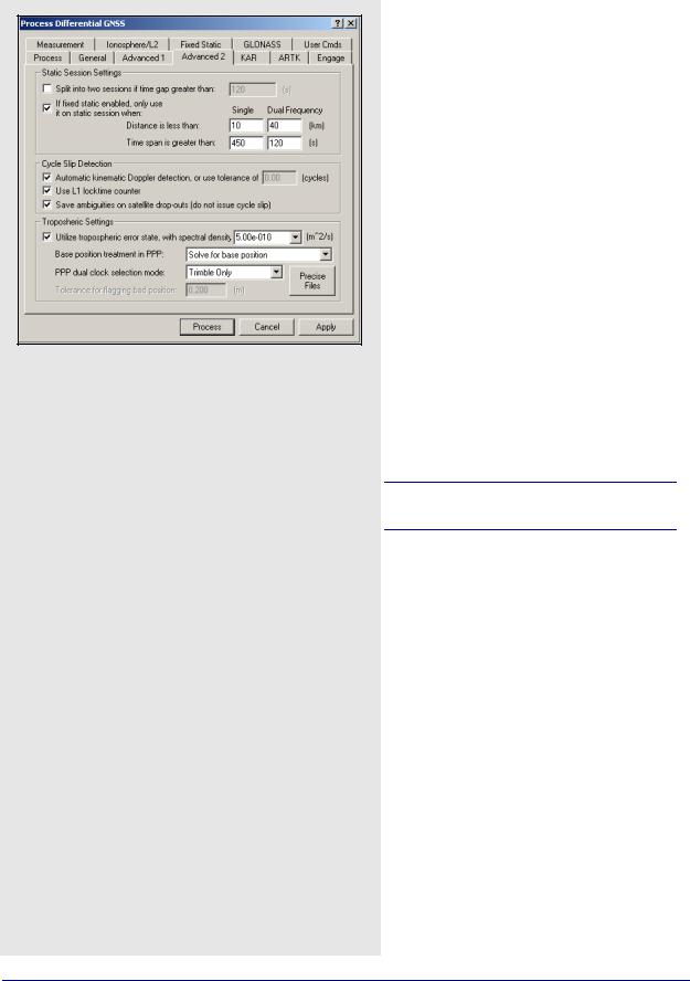
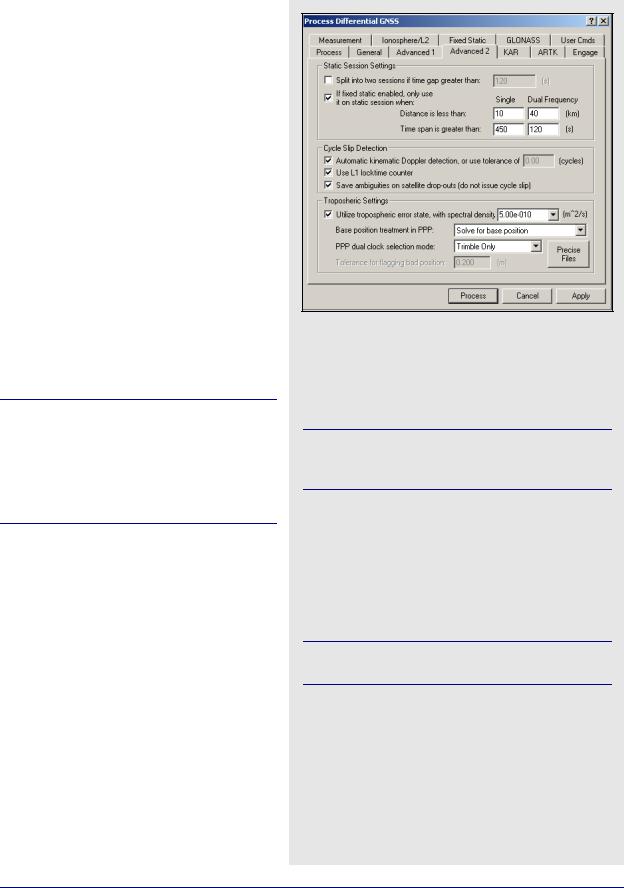
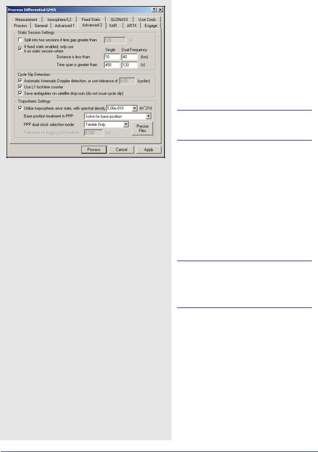
Advanced 2 Options
Static Session Setting
These parameters govern how GrafNav processes static baselines. The options for this setting include the following:
Split into two sessions if time gap greater than
If selected, GrafNav treats time gaps greater than the tolerance as an indication of a new station occupation. This setting is useful if the raw GPS data contains no kinematic epochs between static sessions. It is also useful if there are some blockages so severe that the receiver outputs no raw data records between static sessions.
If fixed static enabled, only use it on static session when
Allows you to specify distance and time tolerances to prevent unreliable static fixes on very long baselines or short time periods. GrafNav computes a fixed static solution for any number of static sessions. Dual frequency has a separate setting option because it sometimes spans a longer distance and requires less data.
For these settings to be applied, Fixed static solution has to be selected on the Process tab.
Cycle Slip Detection
GrafNav uses the locktime read or the computed locktime in the decoder combined with a Doppler check to detect L1 phase cycle slips.
Automatic Doppler tolerance for kinematic detection
This option computes a conservative tolerance based on the data and can be manually set if you are experiencing incorrect cycle slip detection. Use the GPB Viewer to re-compute the Doppler before you use this tool.
68 |
GrafNav / GrafNet 8.10 User Guide Rev 4 |
GrafNav |
Chapter 2 |
|
|
|
|
Use L1 locktime counter
In kinematic mode, the locktime cycle slip check uses flags generated by the GPS receiver to count the L1 locktime. Normally, this should be enabled.
Save ambiguities on satellite drop-outs
Due to serial data errors, some receivers drop satellites without a loss of lock occurring. Without this setting enabled, these drop-outs are treated as a cycle slip. Enabling this setting is especially beneficial for Ashtech receivers. In some cases, however, it is better to interpret this loss of lock as a cycle slip. A good indicator that this checkbox should be disabled is if a filter reset message follows the message “Prn # dropped out for n seconds on b/l ??? -- will try to save ambiguity” in the message log.
Tropospheric Settings
Utilize tropospheric error state, with spectral density
The processing engine adds a tropospheric error state to the Kalman filter.
This option is only recommended for high altitude (vertical separation between base and rover is at least 1000m) or long distance data sets (baseline length exceeds 60km) that are 2 hours or longer. Using it on other data sets may increase the noise in the solution.
Removing the tropospheric error bias is done in two steps. In the first step, GrafNav uses the PPP processor to solve for the tropospheric zenith path delay at all base stations. This is done by either fixing the base station coordinates or by letting the PPP processor solve for them. See the Base position treatment in PPP option below. The second step is the addition of a tropospheric error state to the Kalman filter. By solving for the base stations tropospheric zenith path delay in the first step, the rover’s tropospheric error bias becomes more observable in the Kalman filter.
Base position treatment in PPP
The settings for this option are listed in the shaded box.
Base position treatment in PPP options
Off, don't use PPP
The base station tropospheric zenith path delay is not computed by the PPP processor.
This can make it difficult for the differential Kalman filter to observe the rover’s tropospheric bias. In the majority of cases, this option is not recommended.
Solve for base position
PPP processes in its typical fashion, treating the coordinates as unknowns.
Fix base position
Holds the user-specified coordinates fixed in PPP, which can potentially improve both convergence and overall accuracy—especially for shorter time spans.
This setting should only be selected if you are very confident in the accuracy of the entered coordinates.
Solve then check base position
PPP solves for the base station coordinates and then compares them against the manually entered coordinates.
GrafNav / GrafNet 8.10 User Guide Rev 4 |
69 |
Chapter 2 |
GrafNav |
|
|
PPP dual clock selection mode
Concerns the use of separate clock states for carrier phase and C/A code measurements. The need for this option has only been observed on Trimble receivers, but users can enable or disable this option for any receiver.
Tolerance for flagging bad position
If the solved position from PPP differs from the user-specified coordinates (via Settings | Coordinates) by the tolerance specified, then an error message is displayed and differential processing is not performed.
This option is available only in conjunction with Solve then check base position under Base position treatment in PPP.
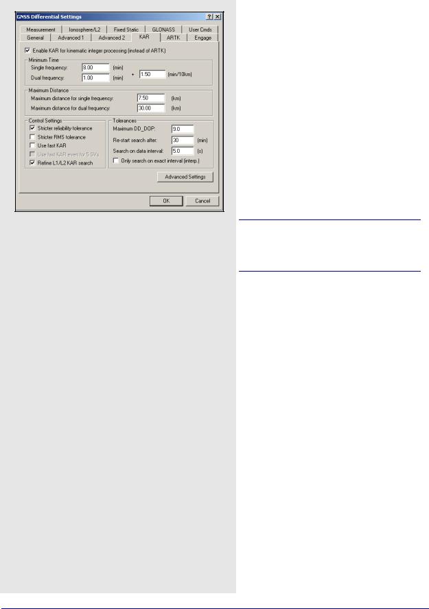
KAR Options
Kinematic Ambiguity Resolution (KAR) is a technique that computes an integer fixed solution of 2 cm while the remote antenna is in motion. Applications of KAR include kinematic initialization and initialization after loss of lock.
Due to the additional measurements present with the L2 phase, KAR solutions that use dual frequency data are considerably more reliable than those using only single frequency data. KAR delivers accurate results with single frequency, but it requires more time.
Both single and dual frequency KAR require at least 5 satellites, but 6 or more are preferable. If KAR fails after a given length of time, it starts searching over again.
As long as KAR successfully resolves, GrafNav restores the ambiguities from the moment it engages so that centimeter accuracies are only unavailable for the actual period of signal obstruction. If no additional complete signal obstructions are encountered following the initial loss of lock and there are good quality phase measurements and low multi-path, then KAR resolves. The FSS or RSS file shows when KAR was engaged and when it was restored. Additional KAR statistics are also shown in this file.
70 |
GrafNav / GrafNet 8.10 User Guide Rev 4 |
GrafNav |
Chapter 2 |
|
|
|
|
Minimum Time
These values represent the minimum amount of time before KAR is invoked and can be customized depending on the type of data available.
In both cases, the values entered are added to the value in the min/10 km input box, which is applied for every 10km of baseline distance. For example, dual frequency receivers with a baseline distance of 20 km, the minimum time required using the default values is the following:
0.5 + [0.5 m * 20 / 10 km] = 1.5 min
Maximum Distance
The distance tolerance for engaging KAR in both single and dual frequency can be defined here. KAR does not engage if the remote is too far from the base station. This improves reliabilities. The default distance is 7.5 km for single frequency and 40 km for dual frequency. These values are designed for a period, like the year of 2000, where the ionospheric activity is high due to solar radiation storms. For later years, these tolerances can be increased.
Control Settings
The following options are available:
Stricter reliability tolerance
The reliability is the ratio of the carrier RMS values between the second-best and best intersections. Larger values means greater reliability. The tolerance for accepting a reliability number is dynamic within GrafNav. This setting adds a bias to the existing dynamic tolerance to make the tolerance strict and reduces the occurrence of incorrect KAR intersections. Be aware that this option can cause KAR to take longer to resolve or not to resolve at all.
Stricter RMS tolerance
This option is similar to the Stricter reliability tolerance but it lowers the tolerance for the RMS value of the best intersection. The tolerance, normally 0.065 cycles, is lowered to 0.05 cycles. The tolerance can also be altered using the KAR_RMS_TOL command. This option reduces incorrect KAR intersections and is usually more effective than the Stricter reliability tolerance option. Both options can also be used at the same time.
GrafNav / GrafNet 8.10 User Guide Rev 4 |
71 |
Chapter 2 |
GrafNav |
|
|
Fast KAR is reliable under the following conditions
•Relatively short master-remote separations (less than 7 km)
•Seven or more satellites in view above a 10-degree elevation mask
•Low multi-path environment
•Clean carrier phase measurements
Use Fast KAR
Fast kinematic ambiguity determination, while not necessary for most GPS work, can benefit certain applications, including the following:
•race car or rocket trajectory determination
•types of surveys under open conditions with scattered obstructions of the sky
•to independently verify a KAR solution if different fixes are obtained in forward and reverse processing.
This option is only available for dual frequency processing because Fast KAR with single frequency data is unreliable.
Be aware of its limitations and know that it is reliable under the conditions listed in the shaded box. In other conditions, consider using ARTK instead.
The Minimum Time defaults under the KAR tab gives enough data to reliably resolve satellite ambiguities under reasonable GPS conditions. In environments with signal obstructions, KAR might not resolve because it could have less data between successive losses of lock than this minimum time. The Use Fast KAR option makes several internal changes to accommodate this, including reducing the minimum KAR time to zero, which tells GrafNav to resolve the ambiguities as quickly as possible. The maximum time before KAR restarts is 8 minutes, which forces KAR to be recomputed more often. This option also increases the amount of data that KAR uses in its computations, reducing the amount of time it takes to resolve.
Use fast KAR even for 5 SVs
Five satellites is the minimum required for KAR computations. It is therefore risky to use Fast KAR in this situation, as it tends to be unreliable. However, given otherwise favorable conditions (see above), it can be used successfully.
72 |
GrafNav / GrafNet 8.10 User Guide Rev 4 |

GrafNav |
Chapter 2 |
|
|
|
|
Refine L1/L2 KAR search
Sometimes, ionospheric noise or carrier multi-path can make it difficult to determine the carrier L1/L2 ambiguities. This setting applies an additional search and leads to faster and more correct ambiguity resolution. This setting also works well in combination with the Stricter reliability tolerance and Stricter RMS tolerance settings. See KAR Options on Page 70.
Tolerances
Maximum DD_DOP
KAR will not search if the DD_DOP is greater than this tolerance. This preserves the reliability of the solution. Raising this value allows KAR to search data that the software would otherwise skip. The default value is 9.
Re-start search after
This is the time length before KAR starts searching over again. Lowering this value causes fixed integer gaps to be lower. This is more practical for dual than single frequency because single frequency KAR needs 15 or more minutes to resolve. The default value is 30 minutes.
Search on data interval
This defines the number of seconds between epochs that KAR uses for processing. If carrier phase errors are random, like in white noise, then using a lower interval improves results, but increases memory usage and computational time. If errors are systematic, like colored/ionospheric noise, than lowering this value has less effect.
Only search on exact interval (interp.)
GPS data can be interpolated with the
Concatenate, Slice and Resample utility or using the Download Service Data feature. In both cases, additional errors of 1 to 3cm can be added to the measurements and is enough to cause KAR not to fix. If this option is enabled and the Search on data interval option has been set to the original source data interval, then KAR is not affected. You can lengthen the minimum KAR time with the KAR tab to use more data, especially if the original interval is 30 seconds or less.
GrafNav / GrafNet 8.10 User Guide Rev 4 |
73 |
Chapter 2 |
GrafNav |
|
|
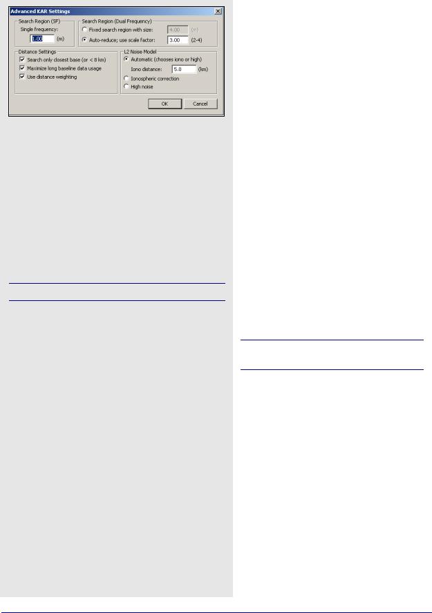
Saerch Region options
Single frequency
The default value is 8 minutes and should not be set to lower than 5 minutes unless azimuth determination is enabled with
a < 2 m distance constraint in GrafMov.
Dual frequency
The default value is 1 minute. You might want to lower this value when fast ambiguity determination is very helpful, an example of this includes urban data. Airborne users with longer baselines might want to increase this number to minimize the effect of the ionosphere.
Fast KAR lowers this to 1 second.
Noise models available for L2
Automatic
This noise model is the default; it chooses between the
High noise and the Ionospheric correction models depending on the current master - remote distance. The distance tolerance can be specified here.
Ionospheric correction
This noise model corrects for the ionosphere and seeds the ionospheric correction algorithms, forming a more accurate KAR fix.
High noise
Places more emphasis on L1 phase (although the widelane is used).
Advanced KAR Settings
Search Region
These setting options relate to the size of the search region used by KAR. The settings are listed in the shaded box.
Distance Settings
Search only closest base (or < 8 km)
This option only applies for multi-base processing. It forces KAR to use the closest base station or those which are closer than 8 km. Disabling it causes all base stations to be used and is normally not desirable. If a certain base station causes suspect fixes due to poor quality data, consider disabling it using the View | GPS Observations | Master | Disable or omitting it from KAR usage.
Maximize long baseline data usage
With this setting disabled, KAR stops using data as soon as the distance between the remote and master is significantly longer than the maximum distance. This can result in minimal data being used, causing lower reliability. With this setting enabled, all usable data less than the maximum distance is used by KAR.
Use distance weighting
KAR has the ability to weight by the inverse of the base-remote distance. This helps with airborne data because the effect of the ionosphere depends on distance.
Baselines shorter than 6 km are not affected.
L2 noise model
KAR supports a number of L2 noise models to determine how GrafNav handles L2 data in KAR. Due to anti-spoofing, L2 can be significantly noisier than L1, and this difference must be taken into account. The noise models that are available for L2 are listed in the shaded box.
ARTK Options
Enable ARTK for kinematic integer processing (instead of KAR)
This option applies the ARTK algorithm to integer ambiguity resolution.
74 |
GrafNav / GrafNet 8.10 User Guide Rev 4 |

GrafNav |
Chapter 2 |
|
|
|
|
General
Criteria for accepting new fixes
Controls how easily the Kalman filter accepts integer fixes generated by ARTK. The levels are listed in the shaded box.
Quality acceptance criteria
This determines how strict ARTK is in signaling a fixed integer solution as a pass. It should be left at Q1, but if ARTK is having trouble computing a fix at all, try Q0. If ARTK is computing many incorrect fixes, try a higher number such as Q2.
Advanced
Only accept fix from closest baseline
Enabling this option results in ambiguities being used only if they were resolved using the closest base station. Best results are obtained with this setting disabled. If enabled, it ignore fixes from farther base stations. If no fix is obtained from the closer base, then a float solution is produced.
Rewind back to time of engagement
If ambiguity resolution is successful, this option fixes the ambiguities starting from the time of engagement. Enabled this option to rewind back to the time of engagement or loss of lock. It should be enabled for most applications. Since rewinding causes fewer satellites used in the restore process, disabling this option often leads to more accurate fixed trajectories but with a larger percentage of the trajectory using a float solution.
Engage Options
These options control when KAR is engaged.
Automatic Engagement
Engage KAR while in STATIC mode:
Engages KAR in static. Be cautious when combining this with the fixed static solution because in certain circumstances, KAR’s solution may supersede that of the fixed solution.
Engage if distance < tolerance1, reset if distance> tolerance2:
This is useful for airborne multi-base processing applications where the aircraft flies over various base stations. It engages the first time that the distance is closer than tolerance1. If the distance becomes greater than tolerance2, a flag is reset and tolerance1 is tested again.
Crteria for accepting new fixes options
Always Accept
Every fix generated by ARTK is applied to the Kalman filter. Since many fixes are duplicates of what has been already applied, using this setting may clutter the Map Window with fix markers.
Strict tolerance
Accept fixes if they are different by 7 mm + 0.4 PPM.
Default tolerance
Accept fixes if they are different by 1.2cm + 0.8 PPM. This setting is suitable for most ground applications
Loose tolerance
Accept fixes if they are different by 4 cm + 1.5 PPM.
On engage only
This level rejects all fixes unless ARTK has been specifically engaged by the user. For airborne, ARTK can sometimes resolve incorrectly due to the long distances and height separation. Therefore, this level is suggested for such applications.
User (+ARTK_AMB_TOL_ command)
Indicates that the tolerances are entered via the ARTK_AMB_TOL command, which can be set under the
User Cmds tab. See User Cmds on Page 84 for more information.
GrafNav / GrafNet 8.10 User Guide Rev 4 |
75 |

Chapter 2 |
GrafNav |
|
|
Engage KAR continuously every:
Engages KAR at a specified interval and is often used for monitoring applications. This value is set around 5 to 20 minutes. Because this mode does not check either baseline distance or data quality, it is the least desirable method for engaging KAR in airborne data.
Engage on event of poor DD_DOP:
4 is the minimum number of cycle slip free satellites need to maintain lock. Even if this minimum is maintained, the geometry can be very poor, as shown by spikes in the Double Difference DOP plot. This option forces KAR to engage after the DOP recovers. The default tolerance is 25.
If the DD_DOP is greater than 100, the epochs plotted because GrafNav skips them. This creates a gap in the data, so check the message logs for these instances.
KAR engages automatically if the DD_DOP is greater than 100.
Manual KAR Engage
Manually engages KAR when it is necessary. For example, when an airborne platform is very close to the base. In this case, consider lowering the minimum KAR time. You must specify the duration as well as the process direction. This feature works well combined with the Manual engage only setting under the Process tab. This allows KAR to engage only at specified times.
76 |
GrafNav / GrafNet 8.10 User Guide Rev 4 |

GrafNav |
Chapter 2 |
|
|
|
|
Measurement Options
Measurement Standard Deviations
Sets the standard deviations of the measurements. These values can be applied to all baselines or can be set individually for each baseline with the Values are for drop-down menu. Baselines altered individually are denoted by an asterisk in the dropdown list. See Chapter 9 on Page 261 for more information on setting these values.
Code
Controls the standard deviation at reference elevation or C/N0 for C/A, P1, and P2 codes.
Carrier phase
Controls the standard deviation at reference elevation or C/N0 for L1 carrier.
Adjust for iono - Adjusts the carrier phase standard deviation for additional error resulting in L1/L2 combination. This option should be enabled.
Doppler
Controls the standard deviation at reference elevation or C/N0 for the Doppler.
Automatic – Sets the standard deviation to 0.25 or 1.0 m/s, depending if the receiver measures Doppler.
The standard deviations are specified here as double differenced values and are at least twice that published by the manufacturer.
Outlier Detection/Rejection
These settings control how the processing engine treats bad satellite measurements using the residuals. The engine rejects measurements based on the number of standard deviations needed to flag an outlier (sigma tolerances). When an outlier is detected, it rejects satellites, measurements or baselines but if too many continuous rejections are encountered, then the software issues a cycle slip to all satellites. This is known as a filter reset.
To control the amount of rejection, select an option in the Level drop-down list. You can enter the rejection and reset values for each measurement or use a stricter phase tolerance to reduce the number of visible spikes in the Carrier Residual RMS plot.
GrafNav / GrafNet 8.10 User Guide Rev 4 |
77 |
Chapter 2 |
GrafNav |
|
|
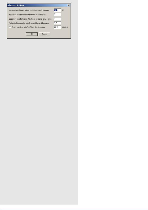
Advanced Settings options
Maximum continuous rejections before reset is engaged
This is the number of seconds of continuous rejections before a reset is issued. Some high data rate kinematic applications may find it appropriate to lower this value.
Epochs to skip before reset induced on code error
On the occurrence of a code error, the processing engine attempts to skip and reject an epoch’s data. This might prevent a reset, but at the expense of a position drop-out. Lower this value to allow fewer missed epochs.
Epochs to skip before reset induced on carrier phase error
This is similar to Epochs to skip before reset induced on code error but applies to the carrier phase. One or two epochs distinguish between one epoch carrier spike, which disappears, and a missed cycle slip, which acts as a step function on the carrier residuals. Only the former can be handled by skipping an epoch.
Reliability tolerance for rejecting satellites and baselines
This is the ratio between the second best residual and the best residual necessary to detect an successful satellite or baseline removal. Generally, this value is left at 4.0, but it can be lowered if a correction is missed or increased if incorrect corrections are occurring.
Reject satellites with C/N0 less than tolerance
This option specifies a threshold below which a measurement is not to be used.
Advanced Settings (for advanced users)
A list of these settings are in the shaded box.
Distance Effects
To properly account for distance dependent error sources, a part-per-million (PPM) value is added to code and carrier phase measurement standard deviations. A PPM is added for the horizontal (spatial) distance and the vertical (height) distance between each master and the remote.
Distance effect amount
High would be used during heavy ionospheric disturbance and would cause a stronger weighting on the nearest base station. The actual PPM values used for each of these levels is determined by the processing engine and depends on the type of processing. Manual distance effects can be entered as well. In this case, you would enter the horizontal and vertical values directly. This effect can be disabled, but this is not suggested, especially for multi-base processing. To view the PPM values used, bring up the Static/KAR Summary file after processing and look for the Dist. Effects field. For very long spatial distances, consider using Low or Very Low. Otherwise, the Kalman filter may destabilize.
Disable baselines when distance becomes greater than "n" km
Use this option when MB processing has many Kalman filter resets or errors. Enabling this option removes a baseline from use during processing if its distance extends beyond the specified tolerance.
78 |
GrafNav / GrafNet 8.10 User Guide Rev 4 |
GrafNav |
Chapter 2 |
|
|
|
|
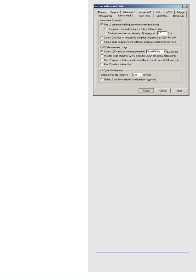
Ionosphere/L2 Options
GrafNav supports full dual frequency processing. For this feature to work, both the master and remote receivers must be dual frequency.
Ionospheric Correction
By making measurements on both L1 and L2, the ionosphere error can be resolved. The effect of the ionosphere under normal conditions and in the absence of ionospheric storms is a relatively small effect at 0.5 to 2 PPM (5 to 20 cm per 100 km). Since L1 and L2 carrier phase need to be combined to remove the ionosphere, the measurement noise increases from sub 1 cm to 1- 3 cm. A further problem occurs because L2 is more prone to cycle slips. Ionospheric correction becomes beneficial on baselines greater than 10 km.
Use L2 carrier for dual frequency ionospheric processing
Two models are available for selection and they are listed in the shaded box.
The distance from the base station when the relative transfer starts can be set using the
Engage distance for relative ionosphere.
This is an advanced parameter and changing it causes little difference in the final solution. You may wish to lower this value during periods of high ionosphere activity.
Correct C/A code for ionospheric using dual frequency data
By combining the C/A code and the P2-code, the ionospheric effect can be removed from the pseudorange measurement. However, this adds additional noise on the order of a few meters. Thus, baselines need to be very long before the effect of the ionosphere is larger than the additional noise induced. Generally, baselines need to be 500 km or more in length.
Correct single frequency using IONEX or broadcast model which must exist
IONEX files contain information relating to the ionosphere on a given day. It can be used with single frequency processing to assist in the ionospheric modeling process. They can be downloaded using the Download Service Data utility. See Section 2.3.8, on Page 38 for more information on how to add precise ephemeris, satellite clock, and IONEX files.
The models for L2 carrier for dual frequency ionopheric processing
Ionospheric Free Model
This can be used for static or kinematic data. This model does a better job of resolving the ionospheric error, but at the expense of being more sensitive to cycle slips. A cycle slip on L2 induces a total cycle slip for that satellite. However, for data sets where L2 is very clean and suffers few losses of lock, this model is strongly suggested. Furthermore, static baselines should use this method, because it aids the fixed static solution if the iono noise model is used. In general, this model works better with most GPS receivers.
Relative Ionospheric Model
This model is normally used for static initialization where the base and remote are close enough that the ionospheric error at that separation can be assumed to be zero. Using the relative transfer algorithm, the ionospheric error is accumulated as the separation grows. If a loss of lock occurs, this transfer cannot continue, and the solution becomes very similar to that achieved using the ionospheric free model. For this reason, the relative model can be used even if the starting point is far from the base. This model is suggested for data with frequent L2 cycle slips.
It is often a good idea to try both models, because one sometimes works significantly better than the other.
GrafNav / GrafNet 8.10 User Guide Rev 4 |
79 |

Chapter 2 |
GrafNav |
|
|
L2/P2 Measurement Usage
The following options are available:
Correct L2C carrier phase using correction
This setting only affects GPS data that is tracking the L2C carrier phase (as opposed to the standard L2P/Y signal). In addition, the GPB data must be the new format and have the L2C flags set on these satellites. Currently, OEMV, Leica 1200 and RINEX v2.11 files are decoded such that L2C satellite tracking registers. For GPS data converted from other formats for example, Trimble, L2C must be registered using the GPS Raw Data Viewer that is, GPBView.
In addition to flagging satellites, the actual correction value must be specified. This value must be correct in order for dual frequency and L2 only KAR processing to succeed. Unfortunately, there are no standards yet and there are several possibilities. Thus far, the following corrections have been observed:
• -0.25
• 0.5
Some manufacturers may choose to align L2C with L2P resulting in a correction of 0.00. For the OEMV, firmware versions 3.0 and 3.1, use 0.5 cycles while future versions (3.2 and greater) will either use -0.25 or 0.00. For Trimble, early versions used 0.5, while later versions will require -0.25.
The simplest way to apply the proper correction is via the decoder which inserts a correction value in the header. This correction value can also be modified or inserted via the Raw GPS Data Viewer.
Using the wrong L2C correction or not having L2C satellites properly registers prevents KAR from successfully computing a fix if L2C signals are tracked. Consider disabling L2C tracking on the GNSS receiver.
80 |
GrafNav / GrafNet 8.10 User Guide Rev 4 |
GrafNav |
Chapter 2 |
|
|
|
|
Process single frequency L2 instead of L1
This mode uses L2 for carrier and P2 for code, and is most appropriate for special applications, including GPS simulator testing, P-Y code receiver testing, and operation of a P-Y code receiver during jamming. For civilian receivers, there is no benefit of this mode of processing.
Use P1 instead of C/A code in the Kalman filter
By default, the processing engine uses C/A code in the Kalman filter. Some receivers deliver better performance if the P1 code is used instead.
This requires the new GPB format. In addition, P1 code data must be present.
Use P2-code in Kalman filter
Under normal circumstances, P2-code measurements are not employed. Enabling this feature adds this measurement to the Kalman filter, thereby possibly improving convergence.
L2 Cycle Slip Detection
The following settings are available:
Small L2 cycle slip tolerance (For advanced users)
KAR and relative ionospheric processing check for small cycle slips on L2 by comparing it against the L1 phase. Raising this value too high increases the chance of detecting a half cycle slip. Lowering this value might cause false cycle slips to be induced from noise. Only advanced users should change this value because it requires the analysis of the results.
Utilize L2 locktime variable if available
The default method of L2 cycle slip detection, which compares L2 against L1, is superior and gives less false detections. You have the option of using the L2 locktime variable. This Variable uses the cycle slip detection of the GPS receiver. If too many cycle slips are being detected, there are many warnings in the message log, assuming the Write cycle slips to message log option is enabled under the Advanced 1 options. The estimated accuracy of the forward or reverse positions might also be higher if ionospheric processing is used.
GrafNav / GrafNet 8.10 User Guide Rev 4 |
81 |
Chapter 2 |
GrafNav |
|
|
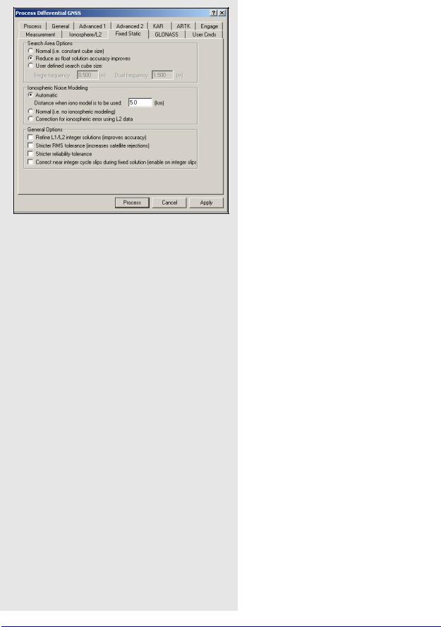
Search Area Option settings
Normal
This uses a constant search region size.
Reduce as float solution accuracy improves
An auto-reducing or adaptive search area is helpful for situations where the fixed solution is failing the reliability tests. Normally, this would be the case on short baselines with single frequency measurements.
User defined search cube size
A user defined search area is not often used. But if the float solution is known to converge very close to the correct solution, then enter zero here.
Ionospheric Noise Modeling settings
Normal
This is similar to the High noise model for KAR.
Correction for ionospheric error using L2 data
This noise model corrects for the ionosphere in its computation. This can improve accuracies, but noise might be higher on short baselines.
Automatic
This noise model chooses between the previous two based upon the distance tolerance entered.
Fixed Static Options
Search Area Options
The search region size can be controlled with the options listed in the shaded box.
Ionospheric Noise Modeling
The ionospheric noise model controls how the L2 measurements are treated in the fixed solution. Due to anti-spoofing, L2 can be noisier than L1. So, on shorter baselines, a noise model placing more weight on L1 that is, Normal L2 Noise, can deliver better results. These options are listed in the shaded box.
General Options
The following options are available:
Refine L1/L2 integer solutions
This setting gets more accurate integer fixes but be aware that it can occasionally hurt the solution.
Stricter RMS tolerance
This option applies a stricter tolerance to the RMS value of the best intersection.
Stricter reliability tolerance
The reliability is the ratio of the carrier RMS values between the second-best and best intersections. Enabling this option applies a more stringent tolerance.
Correct near integer cycle slips during fixed solution
Carrier phase cycle slips are capable of nearing one or more integers. This can also be determined in static mode. In cases where the cycle slip real value is within 0.035 cycles of an integer, the fixed static solution can correct for this integer bias in future raw measurements, improving accuracies. Sometimes the computed cycle slip is close to integer, but the actual cycle slip is a noninteger value. This results in biased measurements that can cause the fixed solution to fail or result in this satellite’s rejection in the NewFixed (multi-satellite) solution.
82 |
GrafNav / GrafNet 8.10 User Guide Rev 4 |

GrafNav |
Chapter 2 |
|
|
|
|
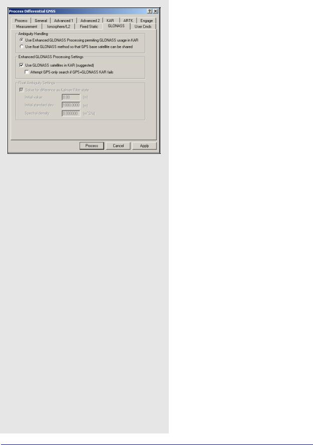
GLONASS Options
The purpose of these settings is to control whether GrafNav utilizes GLONASS using the old-style float ambiguities or the enhanced GLONASS processing. The advantages and disadvantages of each are listed in the shaded box.
Ambiguity Handling
The carrier phase ambiguities associated with the GLONASS measurements can be handled one of the following two ways:
Use enhanced GLONASS processing permitting GLONASS usage in KAR
By using a separate GLONASS base satellite, GLONASS satellites now have the ability to be used in KAR, while trajectories can be cleaner on longer baselines utilizing ionospheric free processing. This mode requires at least two GLONASS satellites(with one as the base).
Use float GLONASS method so that GPS base satellite can be shared
Converts GLONASS measurement to GPS wavelengths which permits a GPS base satellite to be used. Use this method if the number of GLONASS satellites is very low because it works with just one satellite.
Enhanced GLONASS Settings
These options are only available if GLONASS integer ambiguities are being solved for.
Use GLONASS satellites in KAR
This option should generally be selected, as solving integer KAR ambiguities also implies using GLONASS in KAR. If GLONASS is hampering KAR, this setting can be disabled.
Attempt GPS-only search if GPS+GLONASS KAR fails
In the event that KAR is unable to resolve integer ambiguities when using GPS+GLONASS measurements, enabling this option will force the software to re-attempt KAR without them. The advantage can be a higher prevalence of fixes, but the benefit of GPS+GLONASS being more robust that is, having few incorrect fixes, is lost.
Float ambiguity processing
Advantages
•Maximizes satellite usage
•Even one or two GLONASS satellite can be very beneficial
Disadvantages
•KAR ignores GLONASS
Enhanced GLONASS processing
Advantages
•GLONASS satellites can be used in KAR resulting in faster and more reliable KAR fixes
•GLONASS processing can be cleaner especially on longer baselines
Disadvantages
•Needs a GLONASS base satellite which effectively reduces satellite count by one
GrafNav / GrafNet 8.10 User Guide Rev 4 |
83 |
Chapter 2 |
GrafNav |
|
|
Float ambiguity settings
Solve for difference as Kalman Filter state
This option forces the time difference between the GPS and GLONASS time systems to be computed in the Kalman Filter. The difference between the two time systems is never more than a few meters. Corrections to the GLONASS pseudoranges are made using this time difference, but the phase measurements are not corrected since they vary only by the change in this difference over time, which is extremely small. Computed ambiguities account for the remaining error. This setting must be enabled for float GLONASS processing to work effectively.
Initial value
If the initial value for the time difference filter state is known that is, from previous processing, it can be set here. If it is not known, you should enter 0.0.
Initial standard dev
This value describes the accuracy of the initial estimate. Generally, a large value, such as 1000.0m, is used.
Spectral density
The spectral density is noise purposely added to the computation of the time difference state. Since both the GPS and GLONASS time systems are very stable,
this number is always small, from about 0.001mm2/s
to 0.01mm2/s. If the spectral density is set too high, then the time difference computed will fluctuate erratically and never stabilize. Unless very long GLONASS occupations are being processed, 0.0 is sufficient. Otherwise, consider entering a very small number here.
Float Ambiguity Settings
These options are only available if GLONASS float ambiguities are being solved for. Generally, leave these settings as-is. Only users with scientific or research applications should use these settings. The setting options are described in the shaded box.
User Cmds
This changes any command that is passed to GrafNav. It can be used to change commands that are set by the other option tabs, or set commands that are not handled by the other option tabs. See Appendix A on Page 291 for a list of commands.
When a configuration file is loaded, all commands that are not handled by the other option tabs appear here. This includes commands that are not supported in the version of GrafNav being used that can easily be deleted here.
84 |
GrafNav / GrafNet 8.10 User Guide Rev 4 |