

GrafNav |
Chapter 2 |
|
|
|
|
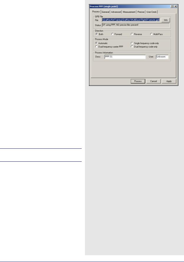
2.5.2Process PPP (single point)
This feature performs precise point positioning (PPP). Base stations are ignored in this mode of processing and only the remote is used. For help adding a remote file to a project, see Section 2.3.7, on Page 37 . See Section 9.7, on Page 275 for background on PPP.
Process
GPB File
File
Indicates the remote observation file to be processed in PPP mode. Click the Info button to open a window that displays the date, time range, and other pertinent information regarding the selected GPB file.
Status
Indicates if single or dual frequency measurements are present and if they will both be used. Also indicates whether or not any precise files have been loaded.
Direction
Both/Forward/Reverse
This setting is much like that of differential processing, where each direction is process independently of each other. It is recommended that you process in both directions, so that the solutions can be combined.
Code-only processing can only be performed in the forward direction.
Multi-Pass
This option processes the data three times sequentially: forwards, reverse, and forwards again. The converged Kalman filter states (position, velocity, tropospheric delay, ambiguities) are preserved after each run and applied to the following run. The result is that improved accuracies are possible for data sets ranging from 1 to 4 hours in length. All the requirements for the default processing style are still applicable here. The final solution is the weighted combination of the reverse solution and the second forward solution.
Process Mode
This setting allows you to choose which measurements you wish to use during processing. The different types of process modes are described in the shaded box.
The different types of process mode
Automatic
If dual frequency data is present, then PPP will be used. Otherwise, single frequency code-only processing is performed.
Dual frequency carrier PPP
This is the preferred method of single point processing, as it has the potential to produce the best results. It requires that carrier phase measurements be made on both the L1 and L2 frequencies.
Single frequency code-only
This method of single point processing is the least desirable. Only the C/A code measurements made on L1 are used. Processing in this mode can only be performed in the forward direction.
Dual frequency code-only
This mode uses the range measurements made on the L1 and L2 bands, and can only be performed in the forward direction.
GrafNav / GrafNet 8.10 User Guide Rev 4 |
85 |
Chapter 2 |
GrafNav |
|
|
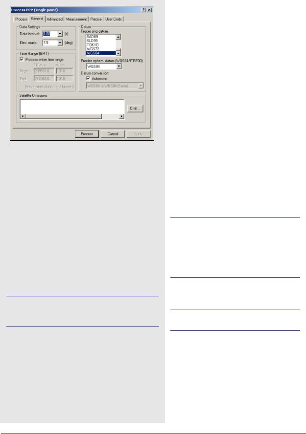
Datum options
Processing datum
The selection made here is dependent on the coordinate system in which the final results are needed. The final trajectory output will be produced in this datum.
Precise ephem. datum
This setting refers to the datum in which the precise ephemeris parameters (SP3 file) are provided. In most cases, the precise files are provided in the ITRF05 datum, which also requires a datum conversion between ITRF05 and the processing datum. If such a conversion is not available, select WGS84.
Datum conversion
The conversion selected here will be dependent on the selections made above. It refers to the conversion used to transform the precise ephemeris values into the processing datum.
PPP uses an absolute datum conversion. This means that any error in the selected datum conversion affects the final trajectory.
Process Information
This box gives you the opportunity to enter descriptive information to help you distinguish this processing run from the others. By default, the software numbers the runs chronologically. You may also choose to provide your name or initials. The information provided here is saved to the Processing History.
General
The following options are available:
Data Settings
Data interval
The interval chosen here depends on whether the data is static or kinematic. For static data sets, use lower intervals such as 10, 15 or even 30 seconds to reduce the effect of time correlation between measurements. If you are processing kinematic data, set this interval at the same rate at which the data was acquired. Avoid data rates of 5Hz or greater due to measurement correlation.
Elev. mask
This value determines the minimum elevation at which a satellite must be in order for its measurements to be used during processing.
Lower values result in the use of noisier measurements due to the greater distance between the satellite and the antenna.
Setting this value too high reduces the number of observations available to the processor, which could be detrimental to the final accuracies.
Time Range
See Time Range on Page 64 for more information.
The H:M:S format is not supported for manual time entry.
Satellite Omissions
See Omit Satellite Info on Page 65 for more information.
Datum
These options are listed in the shaded box.
86 |
GrafNav / GrafNet 8.10 User Guide Rev 4 |
GrafNav |
Chapter 2 |
|
|
|
|
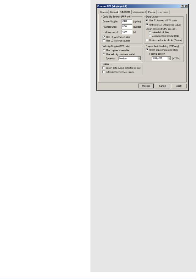
Advanced
Cycle Slip Settings (PPP only)
Coarse/doppler
Use Doppler data to check for large cycle slips. Increase this value if Doppler measurements have large errors.
Fine tolerance
Looks for small cycle slips by comparing L1 against L2.
Locktime cut-off
If the locktime value for measurements on L1 or L2 is less than the value specified here, the satellite is ignored by the processor.
Use L1 locktime counter
This setting determines whether or not to use the L1 locktime values generated by the receiver to detect cycle slips. It should generally be left enabled. Instances where false locktime resets are being recorded may require that this option be disabled.
Use L2 locktime counter
The same as above, but with respect to the L2 locktime counter. It is disabled by default, as the fine cycle clip detector tends to be more reliable.
Velocity/Doppler
Use doppler observable
Enabling this option allows the processor to use the Doppler measurements found in the GPB file for velocity determination.
Use velocity constraint model
If you do not wish to use the Doppler measurements from the GPB file, apply one of the constant velocity vehicle dynamic constraints listed in the shaded box.
Data Usage
Use P1 instead of C/A code
See Use P1 instead of C/A code in the Kalman filter on Page 81 for more information.
Only use SVs with precise values
When precise ephemeris or clock values are not available for all satellites, enabling this option excludes them from processing. This option should be left enabled for best results.
Obtain corrected GPS time via…
Solved clock bias - Use the solved clock bias to compute the corrected GPS time.
GPB File - Use the corrected GPS time as it appears in the GPB file.
Velocity vehicle dynamic constraints
High
Vehicle dynamics (100 m position error due to velocity change)
Med
Vehicle dynamics (10 m position error due to velocity change)
Low
Vehicle dynamics (1 m position error due to velocity change).
GrafNav / GrafNet 8.10 User Guide Rev 4 |
87 |
Chapter 2 |
GrafNav |
|
|
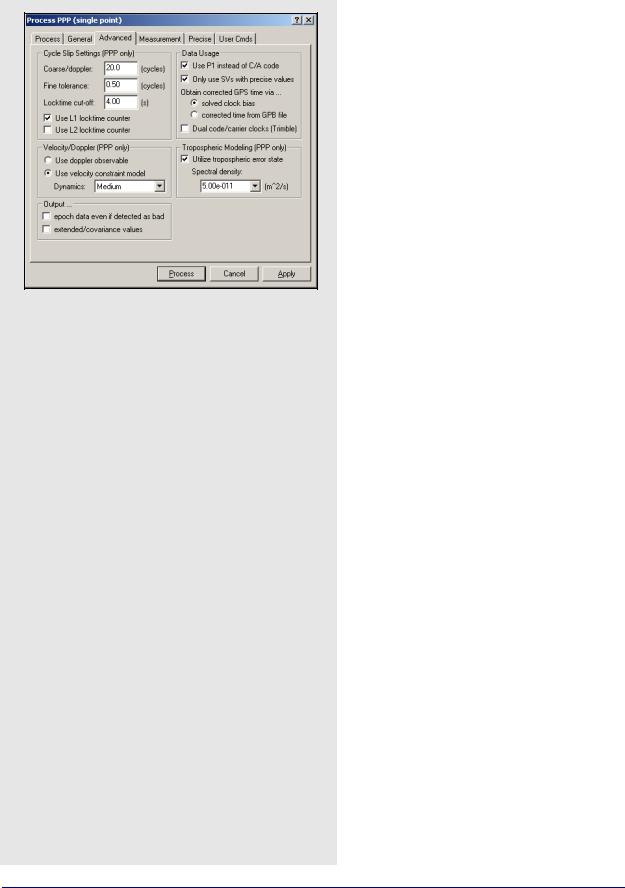
Dual code/carrier clocks.
This option enables or disables the use of separate clock states for the carrier phase and C/ A code measurements. It will likely need to be enabled for Trimble users.
Output
Epoch data even if detected bad
See Write epochs containing bad data on Page 67 for more information.
Extended/covariance values
Enable this option if you wish for the position and velocity covariances to be written to the PPP trajectory files.
Tropospheric Modeling
The PPP processor models the tropospheric zenith delay as a state in the Kalman filter. The tropospheric state can take 30 minutes or longer to converge. Increase the spectral density to allow more room for change within the tropospheric state. For the best processing results, it is recommended that this option be left enabled.
88 |
GrafNav / GrafNet 8.10 User Guide Rev 4 |
GrafNav |
Chapter 2 |
|
|
|
|
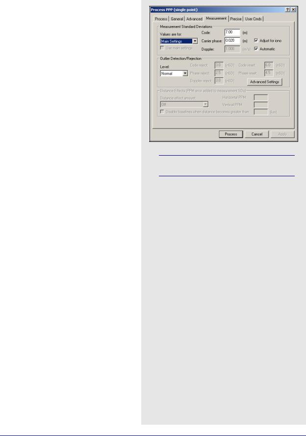
Measurement
Measurement Standard Deviations
Sets the standard deviations of the measurements.
Code
Controls the standard deviation at reference elevation for C/A and/or P1 codes. The default is 7.0 m.
Carrier phase
Controls the standard deviation at reference elevation for L1 carrier.
Adjust for iono – Adjusts the carrier phase standard deviation for additional error resulting in L1/L2 combination. This option should be enabled.
Doppler
Controls the standard deviation at reference elevation for the Doppler.
Automatic – Sets the standard deviation to 1.0 m/s.
Outlier Detection/Rejection
See the Outlier Detection/Rejection on Page 77.
The Satellite Weighting Mode and Distance Effects are not applicable in PPP.
GrafNav / GrafNet 8.10 User Guide Rev 4 |
89 |
Chapter 2 |
GrafNav |
|
|
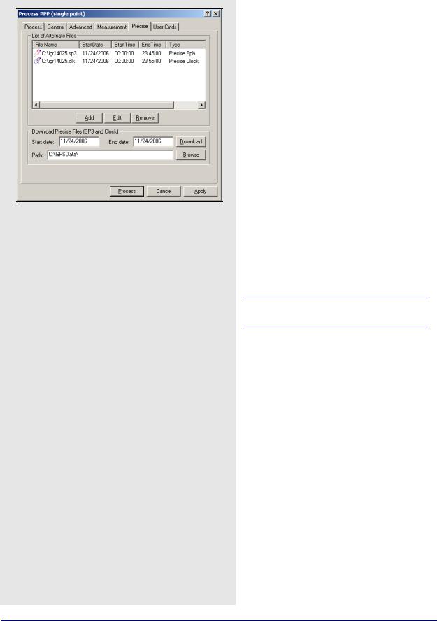
Precise
List of Alternate Files
This tab gives you the opportunity to add or remove any required precise files for the project. It is used to add precise clock (CLK) or ephemeris (SP3) files, but it can also be used to add IONEX (yyi) and broadcast ephemeris (EPP) files, if need be. Once the files have been included in the project, via the Add button, they appear in the window, alongside information regarding the time span that they cover. To disable the use of any of these files without removing them from the project, use the Edit button.
Download Precise Files
A portion of the Download Service Data utility has been integrated here to allow you to download the precise CLK and SP3 files. You need only specify the range of days for which the data has been collected, in MM/DD/YYYY format, and click the Download button. The files are downloaded and saved to the directory specified via the Browse button.
User Cmds
See User Cmds on Page 84 for more information.
PPP commands always start with the prefix “PPP_”.
90 |
GrafNav / GrafNet 8.10 User Guide Rev 4 |