

Chapter 3 |
GrafNet |
|
|
3.4.4 Unignore All Sessions
This feature changes the status of all ignored sessions from Ignore to the status they had previously.
3.4.5 Compute Loop Ties
In some cases, the Traverse or Network residuals shows a poor fit. The first step is to ensure that the network is minimally constrained, which means that there should only be one 3-D control point, or one horizontal and one vertical point. Convert any additional control points to check points. See Section 3.3.8, on Page 157 or Section 3.6.6, on Page 172 for help.
For a constrained network, the poor fit indicated by large residuals can be caused by the following two issues:
• Incorrect antenna heights used for multiple occupations of a point
• Baseline solution is incorrect (by far the most common cause)
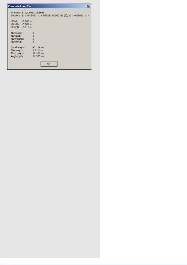
In some cases, it is obvious from the traverse output which baseline is the culprit, but often, further investigation is required. The Compute Loop Tie feature makes such examinations much easier. By adding the vectors of a loop within the network, discrepancy values are formed in the east, north and height directions. For a loop without problems, these values should be near zero. If not, then one of the baselines forming the loop has an error. Loops can be formed in the following two ways:
• Selecting stations of vertices
• Selecting baselines forming legs of loop
Make the selections on the map or by selecting stations or sessions in the Data Manager window. After selecting the first station or session, hold down the Ctrl key while selecting the remaining ones. Selection must be continuous, but it does not matter if the loop is formed in the clockwise or counterclockwise direction. Once a complete loop is formed, select Process | Compute Loop Tie or right-click on one of the selections in the Data Manager window and select Compute Loop Tie. A window containing various statistics for the closed loop will be displayed.
164 |
GrafNav / GrafNet 8.10 User Guide Rev 4 |
GrafNet |
Chapter 3 |
|
|
|
|
3.4.6Network Adjustment
This option invokes the network adjustment contained within GrafNet. External network adjustment programs, such as GeoLab, also support GrafNet's output format.
The network adjustment is only available within GrafNet, and it is a means to more accurately compute each station’s coordinates given the solution vectors computed for each session / baseline. Such an adjustment uses the X, Y and Z vector components, and also utilizes the 3 x 3 covariance matrix which is the standard deviation values + coordinate-to- coordinate correlation. Using least squares, the errors are distributed based on a session’s estimated accuracy. More weight is placed on sessions with lower standard deviations.
Advantages
In the traverse solution, each station’s coordinates are determined using one session from one previous station. For networks with redundant measurements, which is usually the case, this can lead to a suboptimal or even erroneous determination of a station’s coordinates. The network adjustment does a much better job of distributing errors than the traverse solution. This makes it less sensitive to errors as long as a session’s estimated accuracy is representative of actual errors. Thus, the network adjustment generally produces more accurate station coordinates.
Another advantage of the network adjustment over the traverse solution is that it assigns a standard deviation to each point. Estimated standard deviations should be used with caution, but they are a good tool for locating outliers. See Section 3.4.2, on Page 162 for more information on scaling standard deviations to match the data accuracy.
Before running the network adjustment, all baselines must have already been processed. Only good (green) baselines will be used, unless otherwise specified with the Utilize sessions labeled ‘BAD’ in network adjustment option.
How to process with the Network Adjustment
1.After successfully processing all of the baselines within GrafNet, access the network adjustment via Process | Network Adjustment.
The network adjustment will only accept session data flagged as Good. Other baselines will be ignored unless otherwise specified with the Utilize sessions labeled ‘BAD’ in network adjustment option.
For the initial few runs of the network adjustment, the scale factor should be set to 1.0. This will not scale the final standard deviations to match observed session vector residuals. See Page 167 for more information.
2.Click Process to compute a network adjustment solution. This will display any errors encountered.
3.If there are any “hanging stations”, which are stations that are not attached to the network or are attached by a Bad baseline, the adjustment will fail. It is possible to change the status of the baseline to Good from the Sessions window in Data Manager.
4.A .net file is created, which can viewed via
Process | View Network Adjustment Results.
The network adjustment must be re-run if you have reprocessed sessions or changed the station configuration.
GrafNav / GrafNet 8.10 User Guide Rev 4 |
165 |

Chapter 3 |
GrafNet |
|
|
How to interpret the output
The network adjustment output is an ASCII file, which can be printed from GrafNet.
Input Stations
This is a list of the control (GCP) and check (CHK) points in the project. Their associated geographic coordinates and standard deviations are also shown.
Input Vectors
This is the ECEF vector components for each session that has a Good status. The lower triangular of the ECEF covariance matrix is shown next to the vector components. The value in brackets is the standard deviation of the ECEF X, Y or Z axis in meters. The covariance values are not scaled by the Scale Factor entered at the start.
Output Vector Residuals
This is the most important section of the network adjustment output. It indicates how well the session vectors fit in the network. The residual values are shown in local level, where RE is the east axis residual, RN is the north axis residual and RH is the Z axis residual. These values are expressed in meters and should ideally be a few centimeters or less. Larger values may be acceptable for larger networks.
In addition to the residual values, a parts-per-million (PPM) value is shown. This indicates the size of the residuals as a function of distance. 1 PPM corresponds to a 1 cm error at a distance of 10 km. The baseline length is also shown in kilometers. Baselines less than 1 km can have large PPM values. This is because other errors such as antenna centering become an influencing issue. This might not indicate an erroneous session solution. The last value is the combined (east, north and up) standard deviation (STD). This indicates sessions that have one or a combination of the following:
•float solution
•poor satellite geometry (that is, high PDOP)
•short occupations
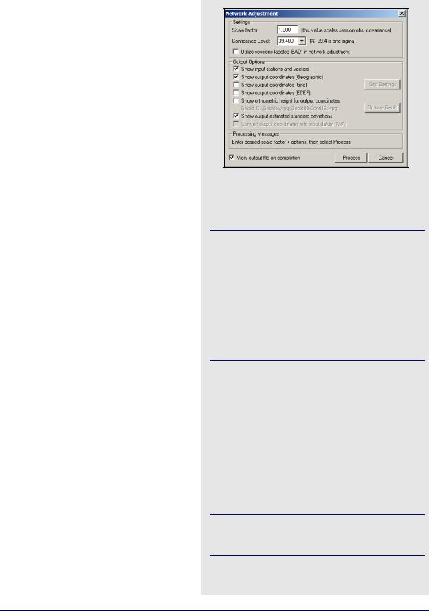
Settings
Scale Factor
Error ellipses should appear on the stations in the Map Window. These ellipses are scaled by this option.
Confidence Level
The level of confidence (in percent) of the error ellipse can also be adjusted. This uses a statistical 2-D normal distribution. Changing this value does not alter the final coordinates, but it will scale the final standard deviations and covariance values. For example, 95% results in a standard deviation scale factor of 2.44.
Output Options
Controls what is output from the network solution.
Show input stations and vectors
Outputs all the control and check points and their vectors. The coordinates are output in geographic form.
Show orthometric height for output coordinates
Requires that you provide a geoid file, which can be selected with the Browse Geoid button.
Other output options include outputting the estimated standard deviations.
To process the network adjustment, press the Process button. This step must be performed each time a project is re-loaded.
View output file on completion option.
Lets you view the ASCII solution file once the adjustment has been made.
Using Multiple Control Points
When multiple control points are present, it is important to initially only use one. This will prevent errors in the existing control from causing otherwise correct session vectors not to fit. Therefore, large tie errors in the traverse solution or large residuals in the network adjustment are attributed to GPS errors.
The variance factor is only truly valid as a scale factor for a minimally constrained adjustment. See
How to interpret the output in the shaded box. Once satisfied with the quality of the GPS data and the fit of the session vectors, you can add additional control points with File | Add / remove Control Points or by right-clicking on a station in the Map Window and selecting Add as Control Point.
166 |
GrafNav / GrafNet 8.10 User Guide Rev 4 |

GrafNet |
Chapter 3 |
|
|
|
|
Since the network adjustment is a least-squares adjustment, it attempts to move control point coordinates to make the network fit better. This is an undesirable effect for many applications. To avoid it, give control points very low standard deviations. The default value is 5 mm, which might have to be lowered if the network fit is poor. Lowering the standard deviation to 0.0001 m forces the control point to “stay put”. A standard deviation of zero is not allowed. Change the standard deviation for control points via File | Add and Remove Control Points. Select the desired control point and click Edit.
Using Horizontal and Vertical Controls
GrafNet supports horizontal and vertical control points in addition to full 3-D control. To utilize this control, you must have available 1-10 m accurate coordinates for the unknown axes (that is, Z for horizontal points and latitude and longitude for vertical points). These coordinates can be obtained from the single point solution (in the absence of SA) or from an initial network adjustment run using just one 3-D control point. The latter method is normally used.
When the vertical and horizontal control points are added, it is important to de-weight the unknown axes. For vertical control points, the horizontal standard deviation is set to 100+ m. For horizontal control points, the vertical standard deviation is set to 100+ m.
Obtain Orthometric Heights
Orthometric heights are available in the network adjustment output.
How to interpret the output cont.
Check Point Residuals
If check points have been added, this section shows how well the known coordinates compare to those computed by the network adjustment.
Control Point Residuals
This section shows the adjustment made to control point residuals. When just one control point is used, then the adjustment will always be zero. With two or more points, the adjustment depends on the input control point standard deviation and the session vector standard deviations.
Output Station Coordinates
This shows the computed coordinates for each of the stations both in geographic and ECEF coordinate systems. The output datum is indicated by the Datum parameter at the top of this file.
The geographic height should be ellipsoidal. However, this is only true if you enter an ellipsoidal height for the control point elevation.
Output Variance / Covariance
This section shows the local level (SE, SN and SZ) standard deviations along with ECEF covariance values. The standard deviation values are scaled by both the input scale factor and the statistical (confidence) scale factor and the covariance values are only scaled by the input scale factor. If error ellipse parameters are desired, then the Write Coordinates feature should be used.
Variance factor
See Page 167 for information.
GrafNav / GrafNet 8.10 User Guide Rev 4 |
167 |

Chapter 3 |
GrafNet |
|
|
Variance Factor and Input Scale Factor
The variance factor is at the bottom of the network adjustment output. It is the ratio between the observed residuals errors and the estimated session (baseline) accuracies. Ideally, the variance factor should be 1.0. This indicates that the estimated errors correspond well to observed errors. A variance factor less than 1.0 indicates that the estimated errors are larger than the observed errors (that is, session standard deviations are pessimistic). Most often, value greater than 1.0 denotes that observed errors are larger than estimated accuracies (that is, session standard deviations are optimistic) exists unless the GPS data is very clean. Thus, low variance factors are normally desired. Very large variance factors 100+ normally indicate abnormally large session errors (that is, a very poor network fit), and you should try and investigate the source of the problem before using the coordinates produced.
The variance factor can also be used to scale the station standard deviations to more realistic values. The network adjustment is initially run with a unity scale factor. The resulting variance factor can then be inserted in the scale factor field from the first screen. After running the network adjustment with this new scale factor, you will notice larger or smaller standard deviations and that the new variance factor should now be ~1.0. This procedure will only work for a minimally constrained adjustment (that is, one 3-D control point, or one 2-D and one 1-D control point).
168 |
GrafNav / GrafNet 8.10 User Guide Rev 4 |