

|
|
|
|
|
392 |
|
SELFISHNESS AND ALTRUISM |
Rationality and Altruism
In Chapter 1, we defined rational in a broad sense as being embodied by preferences that are complete and transitive. Completeness simply means that given the choice between any two states of the world, s1 or s2, one either prefers s1, written s2 s1, or prefers s2, s1 s2, or one is indifferent between the two, written s1  s2. Transitivity requires that for any three options s1, s2, and s3, preferences must be such that if s1 s2 and s2 s3 then s1 s3. If transitivity is violated, then we could devise a money pump by asking a person to pay to cycle among each of the three choices. If a person satisfies these two requirements, we can represent her preferences as a utility function, u
 s
s , that assigns a real value number to each state of the world s, where the person behaves so as to maximize the utility function over the set of available choices.
Altruism does not imply any violation of either of these rules. Define v s
s as the utility function representing the well-being of some other person (not the decision maker) contingent on the state of the world. We may then represent an altruistic decision maker as having preferences embodied in a utility function of the form u
 s, v
s, v s
s , where u
 ,
, is increasing in v
 . Here the impact of the first argument of the utility function may be thought of as the decision maker’s utility of own consumption, and the impact of the second argument as the utility derived from the other person’s well-being. For this to satisfy rationality would require that both people have complete and transitive preferences.
This approach might become clearer if instead of defining utility in terms of states of the world, we define utility based on consumption of some aggregate good x. First, let utility of the other person be given by v x
x , where v
 is increasing in x. Then, where x1
represents the amount of own consumption of good x, and x2 represents the amount of the other person’s consumption, we can represent the state of the world as x =  x1, x2
 , and define U
 x1, x2
 u
u x, v
x, v x
x . Thus, we may denominate the decision maker’s utility of the second person’s preferences in terms of x2, simplifying the model. Let x2 be the amount the second person would consume without any transfer of wealth from the first person. Thus, the decision maker would solve
maxx1,T U x1, |
|
2 + T |
14 1 |
x |
|||
subject to the budget constraint |
|
||
p x1 + T ≤ w1, |
14 2 |
||
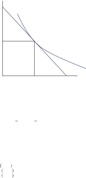
where p is the price of good x, w1 is the amount of wealth available to the first person, and T is the amount of consumption transferred to the second person from the decision maker. Note that this problem is identical to the simple two-good consumer problem introduced in the first chapter, except that both goods have the same price. The solution to this problem occurs where the marginal utility of own consumption is equal to the marginal utility to the first person of the second person’s consumption. In other words, when consuming the optimal bundle, the first person should be indifferent between an additional unit of own consumption and an additional unit of the other person’s consumption. Figure 14.1 displays the solution as the tangent point between an indifference
|
|
|
|
Rationality and Altruism |
|
393 |
|
x2
T *
|
U = U (x1* , x2*) |
FIGURE 14.1 |
|
T = (y − px1)/p |
Utility Maximization with Altruistic |
|
|
|
x1* |
x1 |
Preferences |
curve and the budget constraint. Note that the budget constraint necessarily has a slope of − 1 because both goods have the same price. It is this slope that ensures that the marginal utility of both goods is equal (see equation 1.6).
Now consider the second person. For clarity in this discussion, let’s refer to the original decision maker as a parent and the second person as the child. Suppose the child has only selfish interests and derives utility only from own consumption, v x2
x2 , where x2 = x2 + T and x2 = w2
 p, and where w2 is the wealth of the child. However, suppose this child has a choice that could affect the wealth of the child and the of parent (e.g., how diligent the child is in the family business). The child could either choose option 1, which will result in w1 = 10, w2 = 10, or option 2, in which w1 = 12, w2 = 9. Which option would the child choose? If both parent and child were selfish, the child would always choose option 1, because it gives the child more wealth and thus more consumption.
If the parent is altruistic, the child might choose option 2 if the selfish child is given more than 1 unit of consumption in return. For example, if the parent’s utility is given by
U x1, x2 |
= x1x2 |
, then marginal utility of the parent’s own consumption is |
|
U1 |
x1, x2 |
= x2, |
and the parent’s marginal utility of the child’s consumption is |
U2 |
x1, x2 |
= x1. |
Thus, the parent will always choose to consume where x1 = x2. Suppose |
that p = 1. In this case, option 1 would result in a total of 20 units being purchased, with x1 = 10 and x2 = 10. The parent decides not to make any transfer to the child because the marginal utility of consumption is already equal for x1 and x2. Alternatively, option 2 would result in a total of 21 units being purchased, with x1 = 10.5 and x2 = 10.5. The parent decides to transfer 1.5 units of consumption to the child in order to equalize marginal utility of own and child consumption. Thus, the selfish child is better off choosing a lower personal wealth if it creates greater wealth for both the parent and child. Thus, the child might appear to behave altruistically, though the true motive for the child’s generosity is pure self-interest.


 . But what if the parents have some misconceptions about the child
 that is strictly less than what she would achieve by making a $40 purchase on her own. In turn, the parents then do not derive the amount of utility they anticipated because
 is lower than they believed it would be. Joel Waldfogel refers to the resulting loss of utility as
 w
w = u
= u w
w . In this case, the solution is w
 w
w = w
= w w
w = min
= min w
w . This utility function essentially suggests that the person is only as well off as the worse off of the two of them. The marginal utility of money given to the one with less is 1, and the marginal utility of money given to the one with more (even if it is the dictator herself) is 0. Thus the best possible outcomes would be an equal division. This is an extreme form of other-regarding preferences, where the pain of anyone is everyone’s pain.
 w
w = w
= w
|
|
|
|
Rationally Selfless? |
|
397 |
|
Table 14.1 Other-Regarding Preferences by Sex
Utility Function |
Male |
Female |
Selfish |
47.4% |
37.0% |
Leontief |
25.3% |
54.3% |
Perfect substitutes |
27.4% |
8.7% |
|
|
|
Source: Andreoni, J., and L. Vesterlund. “Which is the Fair Sex? Gender Differences in Altruism.” Quarterly Journal of Economics 116(2001): 293–312.
the percentages of each sex whose preferences most resemble each of these utility functions. A plurality of male participants are selfish in their preferences, and the majority of female participants display Leontief preferences. Female participants in this experiment tend to derive the most utility when consumption is evenly divided between themselves and others. Interestingly, a larger percentage of male participants consider consumption by others to be a perfect substitute with their own consumption. In all, female participants were 10 percent more likely to regard others’ preferences. Similar results have been found by other researchers in variations on the dictator game, suggesting that while women on average are just slightly more altruistic, the nature of their altruism is very different from that seen commonly among men.
Rationally Selfless?
Although altruistic behavior is clearly outside the realm of the majority of economic models, it is unclear whether the altruistic behavior commonly observed in the laboratory or the field is irrational. Using the same data set already described, James Andreoni and John Miller created a series of tests for rational behavior. To test for rationality, we must define some notion of rationality. Each of the tests used by Andreoni and Miller essentially looks for violations of various forms of transitivity using revealed preference. People reveal their preferences when they make a choice among some set of choices. The chosen bundle of goods must yield at least as much utility as any of the forgone options. Economists can then use the revealed preferences from several choices to see if transitivity is violated. Several definitions are helpful. Directly revealed preferred and indirectly revealed preferred states are defined as follows:
Directly revealed preferred: The state s1 is directly revealed preferred to s2 if s1 is chosen when s2 is in the set of available choices.
Indirectly revealed preferred: If s1 is directly revealed preferred to s2, and s2 is directly revealed preferred to s3, and s3 . . . to sT − 1, and sT − 1 is directly revealed preferred to sT , then s1 is indirectly revealed preferred to sT .
The available choices discussed here are the possible divisions of money between the dictator and her counterpart. In this case, people were allotted tokens that could be used to buy points. Each point was worth $0.10. The price of a point ranged from one to four tokens in the experiment, with relative prices for own and other consumption ranging from 1/3 to 3. The participants were also given various endowments of tokens. The endowment of tokens for a single decision ranged from 40 tokens to 100 tokens. This
 , the decision maker will not choose
  in the other.
 . Presented the next time with the same budget set, the person may choose
  , thus violating WARP. If, instead, the indifference
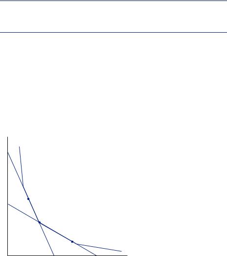

 and chose
  , so that
  is directly preferred to
 ,
, 
 the individual chose
  , so now
  is directly revealed preferred to
  . Finally, suppose that given the possible choices

 , the dictator chose allocation
  is indirectly preferred to
  was available, and
  is directly preferred to
|
|
|
|
|
400 |
|
SELFISHNESS AND ALTRUISM |
set B1 may choose w, making w directly revealed preferred to w . The same person presented with budget set B2 may choose w
 , making w
 revealed preferred to w
 , and making w indirectly revealed preferred to w
 . However, if the person is given the choice between just the two allocations w and w
 , she may choose w
 because they yield the same utility, violating SARP. This leads us to an additional definition of preference relative to a budget constraint, strictly revealed preferred.
Strictly revealed preferred: An allocation w =  w1, w2
 is strictly revealed preferred to w =
  w1, w2
 if it is directly revealed preferred and if p1w1 + p2w2 < p1w1 + p2w2.
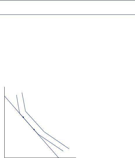
Thus, a bundle is only strictly revealed preferred to other items that were available, but it did not lie on the boundary of the same budget set.
For example, in Figure 14.4, if chosen, w would not be strictly revealed preferred to w , but it would be strictly revealed preferred to w
 , which is interior to the budget constraint. In this case, a rational person for whom greater amounts of both goods results in higher utility could never choose w
 when w was available. If w
 somehow happened to lie along the same indifference curve as w, then there must be some other indifference curve that yields higher utility that lies to the right of w
 and that meets the budget restriction. This is the case if indifference curves are not fat—in other words, if increasing the amount of both w1 and w2 always results in a higher utility. Indifference curves can only have width (and thus be fat) if increasing the amount allocated to both w1 and w2 results in no change in utility for at least some allocation in the set of possible allocations, a situation covered by the generalized axiom of revealed preference (GARP).
Generalized Axiom of Revealed Preference
If s1 is indirectly revealed preferred to s2, then s2 is not strictly directly revealed preferred to s1.
GARP implies that preferences are transitive, and thus rational, but it allows some violations of SARP. Participants in Andreoni and Miller’s study faced eight different combinations of budgets and relative prices. With 176 participants, this produced a total of 1,408 choices. Of the 176 who participated, only 18 (about 10 percent) violated GARP, SARP, or WARP, with a total of 34 choices that violate one of the axioms, though some of the choices violated more than one of the axioms. In total there were 34 violations of SARP, 16 violations of WARP, and 28 violations of GARP. If people made choices totally at random, we would expect 76 percent of the subjects to violate at least one of the axioms of revealed preference. Thus, it appears that the participants in this experiment behaved very close to rationally in this transparent dictator game, though they displayed characteristics of altruism. Moreover, those who violated the axioms made choices that were very close to other choices that would have satisfied the axioms. In other words, some of the apparent irrationality might have been simple mistakes or approximation error.
|
|
|
|
Rationally Selfless? |
|
401 |
|
Thus, while altruistic behavior may be outside the purview of Homo economicus, it does not fall outside the realm of rational decision making. This is not to say that all altruistic behavior is rational. Certainly under the conditions that would create preference cycling, altruistic behavior is also likely to display violations of rational preference axioms. However, under transparent choice decisions, we are as likely to see rational altruistic behavior as we are to see rational behavior in situations where altruism is not an option. More generally, GARP, SARP, and WARP have been used to look for rationality of consumers using data from real-world purchases (e.g., grocery store purchases). In many instances, it appears that consumers violate these notions of transitivity. However, when we apply transitivity to field data, we must recognize that we often cannot observe changes to the budget constraints or other shifting factors that make true comparison of available options and chosen bundles possible. Controlled laboratory experiments such as those conducted by Andreoni and Miller provide a much cleaner test of rational preferences.
 EXAMPLE 14.3 Unraveling and Not Unraveling
One of the primary reasons economists generally suppose people are purely selfish is because it leads us to such simple predictions. In the field of game theory, we typically describe each possible outcome of the game in terms of payoffs, which are meant to be actual measures of utility rather than dollar rewards that one might derive utility from. Unfortunately, when we go to the laboratory or the field to test the predictions of our theory, we cannot easily assign or observe someone’s utility.
Consider for example, the two-player take-it-or-leave-it (TIOLI) game (also called the centipede game) displayed in Figure 14.6. This is a sequential move game, in which each node (where two branches of the game intersect, represented by a black circle in the figure) represents a decision to be made by the player, indicated by the number above the node. Thus, in the first period, Player 1 can either decide to take it (labeled “T” on the diagram) and end the game, or leave it (“L”) and continue the game. If Player 1 chooses T, then Player 1 receives a payoff of 0.40 and Player 2 receives a payoff of 0.10, and the game is over. If Player 1 chooses L, then in the next period, Player 2 can choose either T or L. If Player 2 chooses T, then Player 1 receives a payoff of 0.20 and Player 2 receives a payoff of 0.80, and the game ends. If instead Player 2 chooses L, then the game continues, and Player 1 gets to make the next decision, and so on until the last node.
1 |
L 2 |
L 1 |
L 2 |
L 1 |
L 2 |
L |
25.60 |
||||||
|
|
|
|
|
|
|
|
|
|
|
|
|
6.40 |
T |
|
T |
|
T |
|
T |
|
T |
|
T |
|
|
|
|
|
|
|
|
|
|
|
|
|
|
|
|
|
0.40 |
0.20 |
1.60 |
0.80 |
6.40 |
3.20 |
|
FIGURE 14.6 |
||||||
0.10 |
0.80 |
0.40 |
3.20 |
1.60 |
12.80 |
|
Take-It-or-Leave-It Game |
||||||
|
|
|
|
|
|
|
|
402 |
|
SELFISHNESS AND ALTRUISM |
|
|
|
|
|
|
In searching for behavioral predictions in games, we generally use the concept of the |
|||
|
|
subgame-perfect Nash equilibrium (SPNE). Let us first review the definition of a strat- |
||||
|
|
egy. A strategy for player i, si, is a list of choices player i plans to make—one for each |
||||
|
|
node in which she has a decision to make. A simple decision for one node (e.g., in period |
||||
|
|
1 choose T) does not constitute a strategy. For example, a strategy for player 1 in this |
||||
|
|
case might be s1 = T, T, L because it lists a choice to be taken at each possible node |
||||
|
|
she might be found in. Note that this strategy indicates that in the first period Player 1 |
||||
|
|
will choose T, in the third period (should the game get that far) she will choose T, and in |
||||
|
|
the fifth period (should the game get that far) she will choose L. Clearly, if Player 1 |
||||
|
|
chooses T in the first period, the game will never get to period 3 or 5. However, a |
||||
|
|
strategy must specify what the player plans to do at each node in which she has a choice, |
||||
|
|
even if she does not expect to arrive at that node. Let πi si S− i |
be the payoff received by |
|||
|
|
player i for playing strategy si, when all other players are playing strategies represented |
||||
|
|
by the symbol S− i. The Nash equilibrium is a collection of strategies S = s1, |
, sn , |
|||
|
|
such that for each player i, πi si S− i ≥ πi si S− i , where S = si |
S− i. Intuitively, the Nash |
|||
|
|
equilibrium is a set of strategies, one for each player, such that each player is maximizing |
||||
|
|
her payoff given the strategies of all others involved. Thus, given the strategies of all |
||||
|
|
others, any single player should not be better off for choosing a different strategy. |
||||
|
|
|
An SPNE is a set of strategies that constitutes a Nash equilibrium in every subgame of |
|||
|
|
the original game. A subgame is any set of consecutive nodes containing the last node |
||||
|
|
of the game. For example, the last three nodes constitute a subgame, but the first three |
||||
|
|
nodes do not. The most common way to solve for an SPNE is to use the tool of backward |
||||
|
|
induction introduced in Chapter 13. If we examine the subgame that consists of the last |
||||
|
|
node (period 6), Player 2 can either choose T, resulting in π1 = 3.20 and π2 = 12.80, or L, |
||||
|
|
resulting in π1 = 25.60 and π2 = 6.40. Player 2 does better by choosing T. Player 1 has no |
||||
|
|
choices in this subgame. Hence s1 = , s2 = T |
is the Nash equilibrium for this sub- |
|||
|
|
game. Thus any SPNE must include a strategy for Player 2 that chooses T in the last period. |
||||
|
|
|
Now let us consider the subgame consisting of the nodes for periods 5 and 6. In this |
|||
|
|
period Player 1 can either choose T, resulting in π1 = 6.40, π2 = 1.60, or L, resulting in the |
||||
|
|
subgame consisting of the node for period 6. Because there is only one Nash equilibrium |
||||
|
|
for the node 6 subgame, Player 1 must choose as if L will result in Player 2 choosing T, |
||||
|
|
with π1 = 3.20 and π2 = 12.80. In this case, Player 1 would do better by choosing T. Thus, |
||||
|
|
the SPNE for the subgame beginning with node 5 is s1 = T |
, s2 = T . Continuing with |
|||
|
|
node 4, and so on to node 1, the SPNE for the game is s1 = T, T, T , and s2 = T, T, T . |
||||
|
|
At each node, the player realizes that she can receive a higher payoff by taking now than |
||||
|
|
by leaving, which would result in the other player taking in the next period. Thus, |
||||
|
|
both players would be better off if they chose L for at least a couple periods before |
||||
|
|
choosing T, but their immediate incentives prevent them from doing this. Rational |
||||
|
|
players shrink the pie in the name of selfishly strategic behavior. There is no credible way |
||||
|
|
(given just the structure of the game) to cooperate to obtain a larger payoff for both. This |
||||
|
|
is called the unraveling effect. |
|
|
|
|
|
|
|
As dismal as this prediction may be, it is not what we tend to observe in experimental |
|||
|
|
games of the same form. For example, Richard McKelvey and Thomas Palfrey ran |
||||
|
|
experiments using this form of the TIOLI involving 58 participants drawn from classes at |
||||
|
|
Pasadena Community College and California |
Institute of |
Technology. Participants |
||

|
|
|
|
Selfishly Selfless |
|
403 |
|
received the specified payoffs in cash. In all, McKelvey and Palfrey observed the game being played 281 times. Of those 281 plays, in only two plays did Player 1 choose T in the first round. In fact, the most likely outcome by far was for the game to end in period 4; about 38 percent of all games observed ended this way. Similar experiments have shown that when pairs play several TIOLI games in a row, alternating roles, substantial numbers never play T. This happens even though no matter how many finite periods it might alternate, SPNE predicts unraveling should reduce us to the same T in period 1 result.
Selfishly Selfless
There are many possible explanations for players choosing L in the early phases of the TIOLI game. One explanation is that people are somewhat altruistic. Recall that although SPNE is based upon the idea that the payoffs are measured in utility, in actuality the experimental payouts are in dollars. It could be that people derive utility not just from their own payment but also from the payment given to their opponent in the game. Thus, perhaps player 1 when facing node 1 would be willing to give up $0.20 in order to give the other player an extra $0.70. In fact, if each player is willing to cut her own payoff by 50 percent in order to increase the other person’s payoff by 700 percent, the implied SPNE would now be s1 = L, L, L
 , s2 =
 L, L, L
 . Thus altruism in this case could help grow the pie to be split between the two players. Consider for an instant a Player 2, who is selfish and believes her opponent to be selfish (and that selfishness is common knowledge). In this case, if the game makes it to node 2, Player 2 must reconsider the behavior of her opponent. Her opponent is clearly not behaving like the rational and selfish person Player 2 anticipated. In this case, Player 2 might consider that playing L would lead to similarly irrational behavior by Player 1 in the future.
Both players do not have to be altruistic in order to reach the later nodes of the game. Consider the possibility that some players are altruistic and some players are not. Let us
define an |
altruistic player as |
one |
who evaluates |
her |
utility according to |
u πi, π − i |
= πi + 0.5π − i, where i |
is the |
altruistic player |
and |
i represents the other |
player. Selfish players value only their own payoff, u πi, π − i |
= πi. Suppose that both |
||||
players may be altruistic, but that neither knows whether the other player is in fact selfish or altruistic. Let us consider how we might solve for the SPNE. Consider again the last node, in which Player 2 can choose either T or L. If Player 2 is selfish, she will certainly choose T, because it gives a payoff that is twice what she would receive otherwise. However, if Player 2 is altruistic, the, payoff for T is u = 12.80 + 0.5 × 3.20 = 14.40, and the payoff for L is u = 6.40 + 0.5 × 25.60 = 19.20. Thus, an altruist would choose L. This seems straightforward.
Now consider node 5. Let us suppose that Player 1 is selfish. In this case, if Player 2 is selfish, Player 1 would want to play T. Alternatively, if Player 2 is altruistic, Player 1 would want to play L, because it would result in a much higher payoff. Unfortunately, Player 1 cannot observe whether Player 2 is an altruist. Player 1 might have some guess as to the probability that Player 2 is an altruist, but Player 1 cannot know for certain. One way to think about the payoff is to suppose that ρ is the probability that Player 2 is an

|
|
|
|
|
|
|
404 |
|
SELFISHNESS AND ALTRUISM |
|
|
|
|
altruist. Then, choosing T at node 5 results in a payoff to Player 1 of 6.40. Alternatively, |
|||
|
|
playing L results in probability ρ of receiving 25.60, and |
1 − ρ of |
receiving 3.20. |
|
|
|
If Player 1 maximizes expected utility, then she will |
choose |
L if ρ25.60 + |
|
 1 − ρ
1 − ρ 3.20 > 6.40, or if ρ > 0.14. In fact, if both players believe that there is something around a 15 percent chance the other is altruistic, it is in their best interest to play L even if they are both selfish until the later stage of the game.
In this case, it is difficult for anyone to discern whether their opponent is selfish or altruistic by their actions. Rather, they can only rule out the possibility that the other is selfish and believes that all others are selfish. Such a player would always take in the first round. Thus, the very fact that there are any altruists can lead selfish players to cooperate and behave as if they were altruistic. In general, behavior that appears to be altruistic may be a result of some unobserved reward anticipated by one or more of the players in the game.
EXAMPLE 14.4 Someone Is Watching You
At first blush, the dictator game seems to be a very powerful test of altruistic preferences. Nonetheless, even in a laboratory, it is nearly impossible to control for all potentially important factors. As previously mentioned, it could be that players in the game are motivated by a belief that they are being observed by a deity and will be rewarded later for their actions. This would be very difficult to control for experimentally. Nonetheless, it is possible to approach some unobserved motivations in the common dictator game. For example, it may be that people are motivated to please the experimenter, whom they might believe will punish them for bad behavior at some point in the future. Many of these experiments are conducted by professors with students as participants. These students might anticipate that professors will form long-range opinions of them based on their behavior in this very short-run experiment. Moreover, it may be that people have simply become accustomed to situations in which their behavior is observed and rewarded. This was part of the motivation behind the experiments run by Elizabeth Hoffman, Kevin McCabe, and Vernon Smith examining the experimenter effect on dictator games.
Hoffman, McCabe, and Smith conducted experiments placing participants in several different versions of the dictator game. In some of their experiments, the experimenter was not in the room with the dictators and could not observe which decisions were made by which participants. In others, the experimenter made a point of receiving the money resulting from the decisions and recording it next to the names of the participants who made the decisions. In each of the conditions, the dictator was asked to allocate $10 between her and her counterpart. When the experimenter could observe the actions of the dictators, more than 20 percent of the participants gave more than $4 to the other player. More than half gave at least $2. Alternatively, when the experimenter was not able to determine who gave how much to whom, around 60 percent gave nothing to their anonymous counterpart, around 20 percent gave more than $1, and only about 10 percent gave more than $4. Clearly, many of the participants were motivated to act as if they were altruistic because the experimenter was observing rather than because they cared directly about the player who would receive the money.


 x, r, c
 =
= x − 10r + c, where x is the size of a home, r is the rank of the size of home compared to others in the town (equal to 1 if Lindsay has the largest house), and c is the amount of other goods consumed. Suppose that all homes in the town are 1,500 square feet. Lindsay is contemplating building either a 3,000-square-foot home or a 5,000-square-foot home. Further, suppose that a unit of consumption costs 1 unit of wealth (denominated in $1,000 units). Then, given that Lindsay maximizes her utility subject to a constraint on wealth, p + c < w, where p is the price of the home, we can determine Lindsay’s willingness to pay to upgrade to the larger home by comparing utility with and without each house. Willingness to pay for the larger house should solve
|
|
|
|
Selfishly Selfless |
|
407 |
|
pays WTP3000 for it. The right side is the utility obtained if Lindsay purchases the 5,000-square-foot house, becoming the owner of the largest house in the community, and WTP5000 is paid. This implies that the additional willingness to pay would be given by WTP5000 − WTP3000 = 5000 −
 3000
3000  15.9. Thus Lindsay would only be willing to upgrade to the larger house if it cost less than $15,900.
Suppose instead that other homes in the town were all 4,500 square feet, and suppose that there are nine other homes in the town. Then, the maximum willingness to pay to upgrade to the 5,000-square-foot home from the 3,000-square-foot home would be given by
3000 − 100 + w − WTP3000 = 5000 − 10 + w − WTP5000 |
14 5 |
because having a 3,000-square-foot home would yield the 10th largest house, but having a 5,000-square-foot home would yield the largest house. equation 14.5 implies WTP5000 − WTP3000 = 5000 −
 3000 + 90
  105.9. Now Lindsay would be willing to pay substantially more ($90,000, to be exact) to upgrade because of the status. The additional utility of having 2,000 extra square feet is only worth $15,900, but the added utility of being the biggest and best leads Lindsay to be willing to spend much, much more.
Suppose it cost $40,000 to increase the size of the planned house from 3,000 to 5,000 square feet. In this case, Lindsay would buy the larger house and take a large cut in consumption. However, this large cut in consumption is not in order to obtain utility of space but to obtain utility of status. Note that if everyone in town had similar preferences, everyone in town could be made better off if all choose smaller houses so long as the rank ordering was maintained. In this case, all residents could maintain their status while reducing their expenditures on housing until marginal expense is closer to marginal utility of use.
Psychologists have used simple questions about personal well-being to find very telling relationships between wealth and well-being. You might expect that peoples’ tendency to compare themselves to their neighbors might lead to a situation such that if one person experiences an increase in income she will believe her well-being has increased, but if everyone’s income increases she will consider herself no better off. Richard A. Easterlin compared surveys of individual well-being in countries experiencing massive growth in the 1960s and 1970s, finding a high correlation between income and well-being in any given country but a relatively low correlation across countries. For decades, this was described as the Easterlin paradox. However, cross-country data in that era were spotty and of relatively low quality, especially for developing countries that could experience such growth. More recently, Betsey Stevenson and Justin Wolfers have examined broader multinational datasets that have been collected much more systematically and have found extremely high correlations between income and well-being at both the individual and national levels. This result does not tell us that relative income doesn’t matter so much as it tells us that absolute income matters a lot in determining individual well-being.
More-definitive evidence regarding the importance of relative income comes from women’s labor-market decisions. Here, economists have found that a woman’s decision to work is highly correlated with the difference between her brother-in-law’s (sister’s

|
|
|
|
|
408 |
|
SELFISHNESS AND ALTRUISM |
husband’s) income and her own husband’s income. Controlling for other factors, if a brother-in-law earns more money than her own husband, the woman is more likely to decide to work outside the home, perhaps to keep up with her sister’s consumption. This effect might also play a role in the low rate of savings observed among Americans relative to the rest of the world. Americans face a much more unequal distribution of income and thus it is very difficult for even middle class people to keep up with their richer peers.
EXAMPLE 14.6 Growing Up Selfish
Economists have often argued that we learn to be rational as we gain experience in the marketplace. Thus, it would seem, adults should behave more rationally considering the additional exposure they have gained in making transactions and bargaining in the real world. William Harbaugh, Kate Krause, and Steven Liday set out to see if children truly develop into something resembling Homo economicus as they mature. Such studies of how decision making changes as children mature is common among developmental psychologists, but it is a true novelty among economists.
They enlisted 310 children in second, fourth, fifth, ninth, and twelfth grades to play the standard dictator game. The game was played with tokens that were worth $0.25 each. Each dictator was given 10 tokens to allot between herself and another child of her age. Both the dictator and her counterpart were anonymous, though children knew that they were playing the game with another child in their class. Recall that adults tend to give their counterpart an average of around $2 in the $10 dictator game. This is similar to the behavior observed in the twelfth-grade participants: They allocated an average of 2.1 tokens to their counterpart. This contrasts sharply with children in grades four, five, and nine, in which the average is less than 1.5 tokens being allocated to the other player. It appears that preteens and adolescents are more selfish than adults. Most selfish of all were those in second grade, who gave an average of 0.35 tokens to their counterpart. In fact, the youngest among those tested appeared to behave more like the predictions common in economic theory—ultraselfish—than the more-mature participants.
Given the structure of their experiments, it is difficult to draw any clear conclusions about how a child’s development relates to the development of altruistic behavior. However, the authors argue that their data suggest that altruistic behavior is ingrained in us culturally in our childhood and that many of the differences in how we behave may be a product of our social relationships in these formative years. The fact that children are more selfish than adults is probably not surprising to anyone outside the field of economics. In fact, we commonly call selfish people childish, and parents work hard to teach their children to think of others. Outside the field of economics, many probably take comfort in the notion that people attaining the age of majority have come to display altruistic attributes. For economists, however, this means more-complicated models are needed to describe those we are most often interested in studying.