

|
|
|
|
|
42 |
|
MENTAL ACCOUNTING |
This chapter discusses the full theory of mental accounting and describes several types of behavior that apparently result from this decision heuristic. In particular, we discuss how income source can determine the types of spending, how individual consumers can rationalize bad investments, and how consumers can group events in their mind to obtain a balanced account. Mental accounting is a procedural rational model of consumer choice in that it tells us what is motivating the consumer to make these choices. Although mental accounting can lead to many and varied anomalous decisions, the model itself is surprisingly similar to the accounting methods used by large firms for exactly the same purposes.
Rational Choice with Income from Varying Sources
Many people take income from a wide variety of sources. Some work several jobs; others operate a business in addition to their regular job. Even if only working one job, people can receive money in the form of gifts or refunds that may be considered a separate source of income. Consider the consumer who faces the consumption problem
max U x1, x2 |
3 1 |
x1, x2 |
|
subject to a budget constraint |
|
p1x1 + p2x2 ≤ y1 + y2, |
3 2 |
where y1 is income from source 1 and y2 is income from source 2. The solution to equations 3.1 and 3.2 can be represented by an indirect utility function. An indirect utility
function is defined as V k, p1, p2

 maxx1, x2 U
 x1, x2
 p1x1 + p2x2 ≤ k
 , or the most utility that can be obtained given the prices and the budget k = y1 + y2.
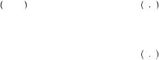
Because utility is only derived from consumption of goods 1 and 2, the particular source of income should not alter the level of utility so long as we remain at the same overall level of income k. Figure 3.1 displays the budget constraints and tangent utility curves under two potential income totals, k1 and k2, such that k1 < k2. The figure shows the optimal consumption bundles under each scenario. Notably, the figure is agnostic about the source of the increase in income. For example, suppose k1 = 100. The particular source of income does not affect the indifference curve. Rather, the shape of the indifference curve is entirely determined by the shape of the utility function, which, as seen in Figure 3.1, is not a function of income source. Increasing y1 by 100 shifts the budget constraint out, so that total income equals 200, resulting in k2 = 200. At this point the consumer will consume more of any normal good and less of any inferior good (the figure displays two normal goods). If, instead, y1 remains at its original level and we add 100 to y2, then we still have a total income of 200, and we remain on the budget constraint given by k2. Thus, although adding 100 to income does alter consumption, it does not matter from which source the added income is derived. All points along the line described by y1 + y2 = k2 will result in an identical budget constraint and result in the same consumption decision. This implies that the indirect utility function increases as income increases. Further, the indirect utility function increases by the same amount, no matter where the additional income comes from.
|
|
|
|
Rational Choice with Income from Varying Sources |
|
43 |
|
x2
U = U(x1 * (k, p1, p2), x2 * (k, p1, p2))
x2 * (k2, p1, p2)
x2 * (k1, p1, p2)
|
|
|
U = V (k2, p1, p2) |
|
|
|
|
|
U = V (k1, p1, p2) |
|
|
|
x2 = (k1 − p1x1)/p |
|
|
||
|
2 |
x2 = (k2 − p1x1)/p2 |
FIGURE 3.1 |
||
x1 * (k1, p1, p2) x1 * (k2, p1, p2) |
x1 |
||||
Income Effects on Consumption |
|||||
The expansion path (the set of points representing the optimal bundle for all possible budget levels) is represented by the curve stretching from the southwest corner to the northeast corner of Figure 3.1 and passing through the tangency points of the indifference curves and the various possible budget constraints. Because utility is independent of the source of income, the expansion path is a single curve that does not depend upon which source of income we may assume the expansion of income is derived from.
Thus, if a consumer behaves according to the standard rational model, any time the consumer receives an amount of money from one source, the additional money results in some change in the consumption bundle the consumer chooses to purchase. If you receive an identical amount of money from any other source (or any combination of other sources), you should alter your purchasing behavior in exactly the same way. By this account, no matter if you receive gift money, hard-earned wages from a job, or a tax refund, you should spend your marginal dollars on the same items. Money is money and should not be treated as a differentiated good.
EXAMPLE 3.1 Food Stamps versus a Cash Payment
The U.S. Supplemental Nutrition Assistance Program (SNAP) was originally introduced as the Food Stamp Program in 1939. The purpose of this program was to provide low-income individuals or families with money to purchase food. Over the course of its history, the program has altered the way benefits were delivered to recipients. Originally, recipients received books of stamps that could be exchanged for food. Currently, recipients are given a card—much like a debit card—that can be used at a supermarket to purchase food.
Historically, most food stamp recipients spent their entire allotment each benefit period and also spent some substantial additional amount from other cash on food.

|
|
|
|
|
44 |
|
MENTAL ACCOUNTING |
Economists have interpreted this to mean that the program, though income enhancing, was not distorting the purchases of participants. If they are spending more than just the food stamp benefit on food, then they should spend the same amount on food if the benefit were given in cash rather than a card that can only be used for food. The standard theory suggests that recipients will spend on food until the marginal utility of food divided by the price of food is equal to the marginal utility of other activities divided by their price (as seen from the discussion on consumer demand in Chapter 1). The only exception to this is seen when this optimal point occurs before the recipient has exhausted the food stamp benefit. Food stamp spending can only include food, and if this point is reached before the benefit is exhausted, then one should still spend the rest of the food stamp benefit, obtaining much more food. If spending the entirety of one’s food stamp budget led to consumption beyond the point where marginal utility of food divided by price was equal to that of other goods, then recipients should not be willing to spend any of their cash on food. This cash could return higher utility by spending on other items.
If people did not spend at least some of their own money on food as well as the SNAP benefit, this would indicate that the program had led them to buy food that they would not have purchased had they been given cash instead. Because food stamp recipients historically spent more than the amount of the benefit that was restricted to food purchases, economists had assumed that this indicated that the food stamp benefit was not leading people to behave differently than they would were we to give them cash, a condition that is important in determining whether there is dead-weight loss from the policy. The notion that cash would be spent the same as a food stamp benefit was tested at one point when the U.S. Department of Agriculture experimented with giving a cash benefit instead of a restrictive benefit card. The original intent of this move was to eliminate the potential stigma associated with participation in the food stamp program. If the program provided cash, no one could tell the difference between someone buying food with food stamp money and someone using money from some other source. Surprisingly, recipients spent substantially less on food when they were given cash instead of a food stamp benefit. Thus, income in cash was being treated differently from income designated as food stamp cash, even though the purchasing power was the same. Clearly, recipients were not finding the point where the marginal utility gained from spending the marginal dollar was equal across activities (in this case, food and all other activities).
EXAMPLE 3.2 Buying Tickets to a Play
Consumers often create a system of budgets for various activities when deciding on consumption activities. Once these budgets are created, they can create artificial barriers in consumption such that the marginal utility gained for the marginal dollar spent on some activities with an excessive budget may be much lower than activities with a lesssubstantial budget. This implies that the indifference curve is not tangent to the budget constraint, as the rational model implies. In this case, consumers could make themselves better off by reallocating money from one budget to the other and approximating the

|
|
|
|
The Theory of Mental Accounting |
|
45 |
|
optimal decision rule embodied by the indifference curve having the same local slope as the budget constraint.
An example of how these budgets can affect behavior was described by Chip Heath and Jack Soll. They asked some participants in an experiment if, given they had spent $50 on a ticket to an athletic event, they would be willing to purchase a $25 theater ticket. Others were asked if they would purchase the theater ticket if they had been given the ticket to an athletic event. A third group was asked if they would pay for the play if they had spent $50 to be inoculated against the flu. Rational decision making should be forward thinking, considering the costs and benefits of the play and not the past spending activities. Interestingly, participants were more likely to turn down the opportunity to attend the play if they had already spent money on the sporting event than if the sporting event were free or if they had spent money on a flu inoculation. Here it appears that having spent money on other entertainment events in the recent past (controlling for any income effects) reduces spending on this category in the future. Alternatively, when the previous entertainment is free, no effect is found. Several other examples are given by Heath and Soll. If consumers consider money to be fungible— easily transferred between uses—then such previous spending should not affect current spending because previous spending is sunk cost. Here we see a very different sunk-cost effect, one that is contingent on budget category.
The Theory of Mental Accounting
At a gross level, mental accounting is a theory of grouping and categorizing money and transactions so that the consumer can systematically evaluate the potential tradeoffs. Spending is categorized into separate budgets for various types of items, such as food in the food stamp example. People can deposit money into separate physical accounts, such as a savings or checking account, and they also treat these as physically different types of money. Income is classified by type (e.g., regular income, bonus, gift). The real workhorse of the theory of mental accounting is that people classify items to allow them to segment decisions. Segmenting decisions allows them to simplify the decision process. Clearly it would be difficult to consider all income, wealth, and transactions at once. By narrowing the items that must be considered when making a decision, people create a manageable problem that can allow better control.
Rather than considering all transactions together to determine the optimal consumption bundle, the theory of mental accounting supposes that people keep a mental ledger of income and expenses by category in their mind in order to keep track of and make spending decisions. Thus decisions may be made either on a categorical basis or on a transaction-by-transaction basis. This ledger can be thought of as a series of accounts with a traditional double-entry accounting system for each account. The double-entry accounting system requires that each transaction be recorded twice: once as a debit and once as a credit. Typically, a business acquires an item; suppose it is a computer costing $1,000. The business needs to keep track of the amount spent as well as the item. The business keeps track of the transaction in books called ledgers, which contain two columns. The left column is for recording debits and the right column is for recording
|
|
|
|
|
46 |
|
MENTAL ACCOUNTING |
credits. The computer is entered in a ledger detailing acquisitions in the left column as a debit of $1,000. The transaction is also written in the right hand of another ledger detailing inventory as a credit of $1,000 worth of equipment. Thus, the process of accounting identifies the gains and losses from each transaction and then records them.
Mental accounting supposes that people open a ledger for each transaction or transaction category, classify each event associated with the transaction as a gain or loss, and seek to have a positive or zero balance by the close of the transaction. Because each transaction is entered in a ledger by itself, decisions are not made on a comprehensive basis but on a piecemeal basis. Thus, food stamp recipients do not determine the optimal overall bundle to consume given their wealth, prices of alternatives, and the amount of food stamps. Instead they might consider the food stamps as a positive entry in their ledger for food purchases, and thus increase their consumption of food by a corresponding amount irrespective of what other alternative uses for the money may be possible.
Because items are evaluated piecemeal based on the category of the transaction, people might behave very differently depending on the source of income or depending on the category of item they consider purchasing. Essentially, a person creates budget categories and evaluates these separately from other budget categories in considering a transaction. Because each income source is categorized, the person fails to treat separate accounts or income sources as completely fungible. Thus money in a savings account is not treated the same as money in a checking account. One may consider one to be more appropriate for a particular type of transaction. For example, one may consider a checking account to be more useful for day-to-day expenses, whereas a savings account is more useful for longer-term holding of money and thus only for more expensive items. Thus, you might regularly spend down the amount in your checking account but loathe to transfer money from your savings account to your checking account, making day-to- day purchasing decisions as if the savings account did not exist.
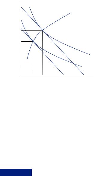
Mental accounting combines this notion of a budget and double-entry accounting with the prospect theory notion of valuing outcomes described in the previous chapter. Each event must be classified as a gain or a loss. Then, the amount is evaluated based on the prospect theory value function as pictured in Figure 3.2. The value function is generally made up of two utility functions: one for gains, ug x
x , and one for losses, ul
 x
x . The value function is concave over potential gains; thus it displays diminishing marginal utility from gains. Thus, the first dollar of gain results in greater pleasure on the margin than the hundredth dollar of gain. As well, the value function is convex over losses, displaying diminishing marginal pain from losses. Thus, the first dollar of loss is more painful on the margin than the hundredth dollar of loss. Additionally, the value function demonstrates loss aversion. This can be seen near the origin as the slope of the utility curve is kinked right at the point between gains and losses, with a much steeper slope for losses than gains. In other words, the consumer considers a marginal loss much more painful than a marginal gain. We typically measure the physical outcomes that make up the argument of the value function, x, either in dollar amounts or in dollar equivalents. Therefore, if you lose $20, then x = −20. If instead you lose basketball tickets that were worth $20 to you, then x = −20 also.
Whether an outcome is considered a gain or a loss is measured with respect to a reference point. This might seem like a trivial task to begin with. For example, if an

|
|
|
|
The Theory of Mental Accounting |
|
47 |
|
Utility value
ug
(losses) |
(gains) |
Dollar value
ul |
FIGURE 3.2 |
The Prospect Theory Value Function |
employee is paid a salary of $70,000, this might form his reference point. Thus, a bonus of $5,000 for a total of $75,000 would be considered a gain. Alternatively, a deduction of $5,000 from the annual pay would be considered a loss. This process is complicated when there are several events to be evaluated at once. Different outcomes may be suggested depending on how items are grouped. For example, a $20 gain and a $10 loss may be coded either as ug 10
10 + ul
+ ul −20
−20 or as ul
 10 − 20
 , depending on whether the events are integrated or segregated. This is discussed in greater detail later in the chapter. If we define our reference point as k, we can define the value function as
ug x − k |
if |
x ≥ k |
v x k |
|
3 3 |
ul x − k |
if |
x < k. |
We often suppress the reference point in our notation by using the form v z
z = v
= v x − k
x − k 0
0 , in which case any negative value is a loss and any positive value is a gain.
The extent to which outcomes are integrated or segregated can be very important in determining the value of a particular transaction or consumption episode. First, consider a man who, after eating dinner at an expensive restaurant, finds that the bill is about $30 more than he was expecting to pay. In addition, suppose he leaves the restaurant and picks his car up at the nearby parking garage and finds that he is charged $4 more than he had expected to pay for parking for the dinner. Here, the amount the man expected to pay serves as the reference point. In each case, the man spent more than he expected, resulting in a loss relative to the reference point. If these expenses are segregated, then he would experience v −30
−30 + v
+ v −4
−4 . Alternatively, if he integrated these expenses, he would experience v
 −34
−34 . He might reason that they were both added expenses of going out to eat and thus treat them all as one loss. He might reason, “I had to pay way too much to go out tonight.” Alternatively, he might separate the experiences because they occurred at different times and in different places. He might reason, “First I was charged
|
|
|
|
|
|
|
48 |
|
MENTAL ACCOUNTING |
|
|
|
|
|
Utility value |
|
|
|
|
|
|
|
v |
|
|
|
v(34) |
|
|
|
|
|
v(30) |
|
|
|
|
|
v(4) |
|
|
|
|
|
−34−30 −4 |
|
|
|
|
|
4 |
30 34 |
Dollar value |
|
|
|
|
|
|
|
|
|
v(−4) |
|
|
|
|
|
v(−30) |
|
|
|
FIGURE 3.3 |
v(−34) |
|
||
|
Integrating or Segre- |
|
|
|
|
|
gating Events |
|
|
|
|
|
|
|
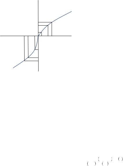
way too much for dinner, and then later I was charged too much to park.” Figure 3.3 |
||
|
|
|
depicts the two possible scenarios. Because the value function over losses is convex, the |
||
|
|
|
$4 loss evaluated on its own is associated with a much greater loss in utility than when |
||
|
|
|
added to the original $30 loss. This means that the person who integrates the two losses is |
||
|
|
|
much better off than the person who segregates the two losses. When they are integrated, |
||
|
|
|
we may say that they are entered into the same mental account. |
||
|
|
|
The same thing happens in reverse for gains. If instead the man had been charged $30 |
||
|
|
|
less than he expected for dinner and $4 less than he expected for parking, he would be |
||
|
|
|
much better off for segregating the gains. Again, Figure 3.3 shows that because the value |
||
|
|
|
function is concave over gains, the pleasure experienced for saving $4 in parking when |
||
|
|
|
evaluated on its own is slightly greater than the pleasure for adding $4 in savings to the |
||
|
|
|
$30 savings experienced when paying for dinner. Thus, the person who segregates |
||
|
|
|
the experiences in this case feels better off than the person who integrates them. |
||
|
|
|
Finally, if a person experiences some gains and some losses, we can make some |
||
|
|
|
further generalizations. For example, suppose the man paid $30 less than he expected |
||
|
|
|
for dinner but found a $30 parking ticket on his car when he left the restaurant. If he |
||
|
|
|
integrated these experiences, he would experience utility of v 30 − 30 = v 0 . Alter- |
||
|
|
|
natively, if he segregates these experiences, he obtains v −30 + v 30 . Because of loss |
||
|
|
|
aversion, the pain from the loss of $30 is greater than the pleasure for the gain of $30. In |
||
|
|
|
this case, the man might feel better off if he integrates the events. This might lead the |
||
|
|
|
reader to believe that a person will strategically choose either to integrate or segregate |
||
|
|
|
events in order to obtain the greatest utility. This possibility is discussed later in |
||
|
|
|
the chapter. |
|
|
|
|
|
The final component of mental accounting incorporates the notion of transaction |
||
|
|
|
utility. People use a value function to assess their consumption experience relative |
||
|
|
|
to their expectations—their consumption utility—but they also use a value function to |
||
|
|
|
assess their enjoyment of the particular deal they were able to obtain—their transaction |
||
|
|
|
utility. Again, this raises the specter of whether a person will integrate or segregate |
||