

|
|
|
|
|
2 |
|
RATIONALITY, IRRATIONALITY, AND RATIONALIZATION |
model and its roots. Rightly, this is the first theory that a behavioral economist seeks to apply when describing individual behavior. It is only when using a rational model becomes impractical or inaccurate that behavioral economists seek alternative explanations. Nonetheless, these alternative explanations may be very important depending on the purpose of the modeling exercise. For example, if, as an individual, you discover that you systematically make decisions that are not in your best interest, you may be able to learn to obtain a better outcome. In this way, behavioral economics tools may be employed therapeutically to improve personal behavior and outcomes. Alternatively, if a retailer discovers that customers do not fully understand all relevant product information, the retailer might improve profits by altering the types and availability of product information. In this case, behavioral economics tools may be employed strategically to take advantage of the behavior of others. An economics researcher might also be interested in finding general theories of decision making that can be applied and tested more broadly. In this case, behavioral economics tools may be applied academically. The motivation for employing behavioral economics, be it therapeutic, strategic, or academic, in large part determines the types of models and phenomena that are important to the interested student. To this end, we employ three types of economic models: rational, behavioral, and procedurally rational. Throughout this book, we use these distinctions in discussing the uses and applications for behavioral economic modeling.
Finally, the roots and history of behavioral economics are inextricably linked to experimental economics. Although this text tries to avoid becoming one on experimental methods, it is important to discuss some of the basics of experimental economics, why it is so useful in behavioral economics, and what this might mean for the wider use of behavioral economic concepts.
Rational Choice Theory and Rational Modeling
Behind every rational model is the notion that people are making optimal decisions given their access to information or the other constraints that they might face in their decisions. The most common rational models used in economics are the utility-maximization model and the profit-maximization model. The utility-maximization model assumes that the person has preferences over choices that can be expressed as a utility function. This function represents the level of enjoyment or welfare the person receives for a set of choices, often thought of as a bundle of goods that can be consumed. For example, a typical model presented in a course on microeconomics might suppose that one can consume two goods measured by the quantities x1 and x2. The person’s decision problem could then be represented as
max U x1, x2 |
1 1 |
x1, x2 |
|
subject to a budget constraint |
|
p1x1 + p2x2 ≤ y, |
1 2 |
|
|
|
|
|
|
|
|
|
|
|
|
|
|
|
|
|
|
|
|
Rational Choice Theory and Rational Modeling |
|
3 |
|
||||||
where U x1, x2 |
is the utility obtained from consuming amounts x1 and x2, p1 is the price |
|
|
|||||||||||
of good 1, p2 is the price of good 2, and y is the total budget that can be spent. The |
|
|
||||||||||||
consumer’s problem in equations 1.1 and 1.2 is to find the consumption bundle |
x1, x2 |
|
|
|||||||||||
that maximizes his utility without exceeding his budget constraint. It is generally |
|
|
||||||||||||
assumed that utility increases as either x1 or x2 increases. Further, the underlying pre- |
|
|
||||||||||||
ferences are assumed to be complete and transitive. By complete, we mean that given |
|
|
||||||||||||
any two possible consumption bundles, x1, x2 and x1, x2 , the consumer prefers |
|
|
||||||||||||
bundle 1, x1, x2 , prefers bundle two, x1, x2 , or is indifferent between the two. No |
|
|
||||||||||||
possible pair of bundles exists for which the consumer has no preference. By transitive, |
|
|
||||||||||||
we mean that given any three bundles, if the consumer prefers x1, x2 |
to x1, x2 |
, and the |
|
|
||||||||||
consumer prefers x1, x2 to |
|
1, |
|
2 , then the consumer cannot prefer |
|
|
1, |
|
2 to |
x1, x2 . |
|
|
||
x |
x |
x |
x |
|
|
|||||||||
Information about the consumer’s preferences over consumption bundles is coded in the |
|
|
||||||||||||
utility function by assigning a higher utility number to any bundle that is preferred or by |
|
|
||||||||||||
assigning an equal number to any bundles to which the consumer is indifferent. |
|
|
||||||||||||
The decision problem can be represented as in Figure 1.1. The consumer can only |
|
|
||||||||||||
consume any point in the triangle with sides formed by the x1 axis, the x2 axis, and |
|
|
||||||||||||
the budget constraint, which is the straight downward-sloping line found by solving the |
|
|
||||||||||||
budget constraint for the quantity of good 2 as a function of the amount of good 1, |
|
|
||||||||||||
x2 = y − p1x1 |
p2. Preferences are represented in Figure 1.1 by indifference curves, |
|
|
|||||||||||
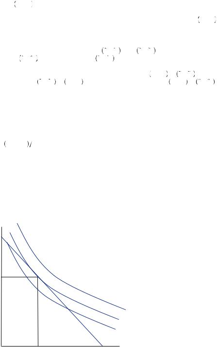
a collection of consumption bundles such that each point in the set results in the same level of utility. Figure 1.1 depicts three indifference curves, each curving to the southeast as one moves down the x2 axis. Indifference curves that are farther to the northeast of the figure represent higher levels of consumption of both goods and thus represent a higher level of utility. The assumption of complete and transitive preferences implies that these indifference curves cannot intersect one another. The intersection of two different indifference curves would require the intersection point to result in two different levels of utility.
x2
x2*
|
U > U(x1*, x2*) |
|
|
|
U = U(x1*, x2*) |
|
|
|
U < U(x1*, x2*) |
|
|
|
x2 = (y – p1x1)/p2 |
FIGURE 1.1 |
|
x1* |
x1 |
||
Utility Maximization |
|
|
|
|
|
4 |
|
RATIONALITY, IRRATIONALITY, AND RATIONALIZATION |
For a full discussion of the utility maximization model, the reader is referred to Nicholson and Snyder or Varian. The consumer problem is to maximize utility by finding the northeastern-most indifference curve that has at least one point that satisfies the budget constraint. This can occur at the intersection of the budget constraint with the x1 axis (where x1 = y p1 and x2 = 0), where the budget constraint intersects the x2 axis (where x1 = 0 and x2 = y
 p2), or at a point such as
  x1*, x2*
 in Figure 1.1, where the indifference curve is tangent to the budget constraint. We call this third potential solution an internal solution, and the first two are referred to as corner solutions. Internal solutions are the most commonly modeled solutions given the mathematical convenience of determining a tangency point and the triviality of modeling single-good consumption. The set of tangency points that are traced out by finding the optimal bundle while varying the total budget is called the income expansion path. It generally reflects increasing consumption as income increases for any normal good, and it reflects decreasing consumption for any inferior good.
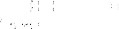
To find the solution to the utility-maximization problem, we must define the concept of marginal utility. The marginal utility of x1, which we denote  U
U x1, x2
 x1, is the amount of utility gained by increasing consumption of x1, or the slope of the utility curve with respect to x1. The marginal utility of x2, denoted
  U
U x1, x2
 x2, is the utility gained from increasing consumption of x2, or the slope of the utility curve with respect to x2. An internal solution to the utility maximization problem occurs where the ratio of the marginal utilities is equal to the ratio of prices:
|
|
|
|
|
|
U x1*, x2* |
|
p1 |
|
|
||
|
|
|
|
|
x1 |
= |
. |
1 3 |
||||
|
|
|
|
|
|
|
|
|
|
|||
|
|
|
|
|
|
U x1*, x2* |
p2 |
|||||
|
|
|
|
|
|
|
|
|
||||
|
|
|
|
|
x2 |
|
|
|
||||
|
|
|
|
|
|
|
|
|
|
|
|
|
Note that − p1 p2 |
is the slope of the budget constraint. The slope of an indifference |
|||||||||||
curve is equal to |
− |
U x1, x2 |
|
U x1 |
, x2 |
. Thus, any point solving equation 1.3 yields a |
||||||
x1 |
|
|
|
|
||||||||
|
|
|
|
x2 |
|
|
|
|
|
|||
point on the indifference curve with the same slope as the budget constraint. If in addition that point is on the budget constraint, p1x1* + p2x2* = y, then we have found the optimal consumption bundle. The Advanced Concept box at the end of this chapter presents a mathematical derivation of this concept for the interested reader.
Rationality and Demand Curves
If we know the functional form for the utility function we can find the marginal utility function. Then we can solve the system of equations 1.2 and 1.3 for a set of two demand functions, x1* p1, p2, y
 and x2*
 p1, p2, y
 , that represent the amount of good 1 and good 2 that will make the consumer as well off as he can possibly be given the prices for the goods and the allocated budget. This model implies a set of relationships between prices and quantities based on the assumption of a utility function and its relationship to the quantity consumed. In particular, one may derive the law of demand—that as the price of a good increases, a consumer will purchase less of that good—which may be useful in pricing and marketing goods. This model makes several assumptions about the structure of the problem that are common among nearly all utility-maximization problems.
|
|
|
|
Rationality and Demand Curves |
|
5 |
|
Foremost among these assumptions is the notion that the consumer has a set of wellunderstood and stable preferences over the two goods. However, simple introspection can lead us to question even the most basic of these assumptions. If consumers have a well-defined and stable set of preferences over goods, then what role can advertising serve other than to inform the customer about the availability or characteristics of a product? Were this the case, advertisements for well-known products should not be terribly effective. However, marketers for well-known products continue to buy advertising, often providing ads that yield no new information to the consumer. Further, consumers are often faced with goods with which they are unfamiliar or have not considered purchasing, and thus they might have incomplete preferences.
The utility-maximization model assumes that consumers know how their choice will result in a particular outcome. It seems reasonable that consumers choosing to buy four apples would know that the result would be their consuming four apples at some point in the future; but they might not know how many contain worms or have irregularities in taste or texture. In fact, consumers seldom face decisions with completely certain outcomes even for the simplest actions. In some cases, the consumer might not even be certain of the possible choices available. In an unfamiliar restaurant, diners might not fully read the menu to know the full range of possible choices. Even if they do, they might not be aware of the menu of the neighboring ice cream parlor and consider only the dessert possibilities at the restaurant.
Finally, the model assumes that consumers have the ability to determine what will make them better off than any other choice and that they have the ability to choose this option. The notion that the consumer can identify the best outcome before making a choice seems counter to human experience. Students might believe they should have studied more or at a different time in the semester, and people often feel that they have overeaten. Where exams and food consumption are repeated experiences, it seems strange that a person would not be able to eventually identify the correct strategy—or lack the ability to choose that strategy. Nonetheless, it happens. Perhaps this is due to an inability to execute the correct strategy. Maybe the spirit is willing but the flesh is weak. Rational models of consumer choice rely heavily on complete and transitive preferences, as well as on the ability of the consumer to identify and execute those preferences. If any of these assumptions were violated, the rational model of consumer choice would struggle to describe the motivation for individual behavior.
Even so, these violations of the underlying assumptions might not matter, depending on how we wish to use the model. There are two primary lines of argument for why we might not care about violations. First, if these assumptions are violated, we may be able to augment the model to account for the discrepancy resulting in a new model that meets the conditions of rationality. For example, if the consumer is uncertain of the outcomes, we may be able to use another rational-based model that accounts for this uncertainty. This would involve assuming preferences over the experience of uncertainty and modeling the level of uncertainty experienced with each good, such as the expected utility model discussed in later chapters, and supposing again that consumers optimize given their constraints and preferences. A second argument notes that a model is designed to be an abstraction from the real world. The whole point of a model is to simplify the real-world relationships to a point that we can make sense or use of it. Thus, even if the assumptions of our model are violated, consumers might behave as if they are
|
|
|
|
|
6 |
|
RATIONALITY, IRRATIONALITY, AND RATIONALIZATION |
maximizing some utility function. Paul Samuelson once compared this as-if approach to a billiards player who, although he does not carry out the mathematical calculations, behaves as if he can employ the physics formulas necessary to calculate how to direct the desired ball into the desired hole. This as-if utility function, once estimated, may be useful for predicting behavior under different prices or budgets or for measuring the effects of price changes. Even if it is only an approximation, the results may be close enough for our purposes.
In truth, the adequacy of the model we choose depends tremendously on the application we have in mind. If we wish primarily to approximate behavioral outcomes, and the variation from the behavior described by the model is not substantial for our purpose, the rational model we have proposed may be our best option. Our reference to a deviation from rational behavior as an anomaly suggests that substantial deviations are rare, and thus rational theory is probably adequate for most applications. If the variations are substantial, then we might need to consider another approach. It is true that many of the applications of behavioral economics could be modeled as some sort of rational process. For example, a consumer might use a rule of thumb to make some decisions because of the costs involved in making a more-deliberate and calculated choice. In this case, the consumer’s cognitive effort might enter the utility function leading to the observed heuristic. The consumer, though not at the best consumption choice given unlimited cognitive resources, is still the best off he or she can be given the cognitive costs of coming upon a better consumption choice. On occasion this is a successful strategy for dealing with an observed behavior. More often than not, however, it leads to an unwieldy model that, although more general, is difficult to use in practice. Occam’s razor, the law of research that states that we should use as few mechanisms as possible to explain a relationship, might compel us to use a nonrational approach to modeling some economic behavior.
If instead, we are interested in the motivation of the decision maker, rather than simply approximating behavior under a narrow set of circumstances, the as-if approach might not be useful. For example, using mathematical physics to describe a pool player’s shots might yield relatively accurate descriptions of the players’ strategy until the pool table is tilted 15 degrees. At this point, the pool player is dealing with an unfamiliar circumstance and could take some significant time learning to deal with the new playing surface before our model might work again.
The need for a simple model drove classical economists to abstract from real behavior by assuming that all decision makers act as if they are interested only in their own wellbeing, with full understanding of the world they live in, the cognitive ability to identify the best possible choices given their complete and logical preferences, and the complete ability to execute their intended actions. Such omniscience might seem more befitting a god than a human being. Nineteenth-century economists dubbed this ultrarational being Homo economicus, noting that it was a severe but useful abstraction from the real-world behavior of humans. Although no one ever supposed that individual people actually possessed these qualities, nearly the whole of economic thought was developed based on these useful abstractions. As theory has developed to generalize away from any one of the superhuman qualities of Homo economicus, the term has become more of a derisive parody of traditional economic thought. Nonetheless, there is tremendous use in this, absurd though it is, starting point for describing human behavior.
|
|
|
|
Rationality and Demand Curves |
|
7 |
|
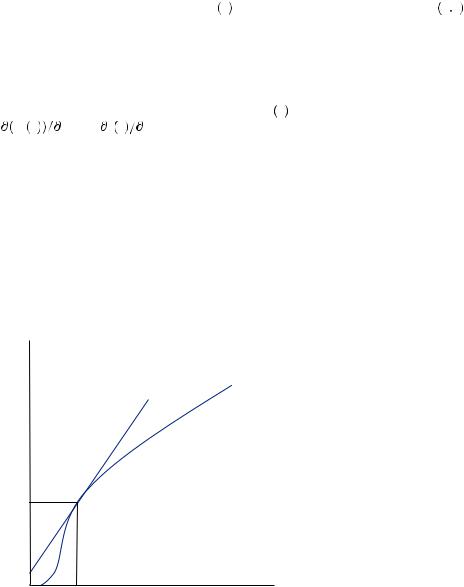
In addition to the utility model, microeconomic theory also hinges very heavily on the notion that firms make decisions that will maximize their profit, defined as revenues minus costs. This is actually a somewhat stronger assumption than utility maximization because it generally specifies a relationship between a choice variable and the assignment of profit, which is generally observable. Alternatively, utility is not observable, and thus it can have an arbitrary relationship to choice variables. For example, a common profit-maximization model may be written as
max pf x − rx − C, |
1 4 |
x |
|
where x is the level of input used in the production process, p is the price the firm receives for output, f  x
x is a production function representing the level of output as a function of input, r is the input price, and C is the fixed cost of operation. To find the solution to equation 1.4, we must define the marginal revenue and the marginal cost functions.
Revenue |
in equation |
1.4 is given by pf x . Marginal revenue, denoted |
pf x |
x = p × f x |
x, is the additional amount of revenue (price times quantity |
sold) that is received by increasing the input, or the slope of the revenue function. Here,  f
f  x
x
 x is the slope of the production function. The marginal cost is the additional cost of increasing the amount of input used, r. The profit-maximization problem is generally solved where the marginal revenue from adding an additional input is equal to the marginal cost of production so long as rent, pf
  x
x − rx, is great enough to cover the fixed cost of operation. Otherwise the firm will not produce because they would lose money by doing so. Marginal cost is equal to marginal revenue where p
  f
f  x*
x*
 x = r, or in other words at the point where a line tangent to the production function has a slope of r
 p. This is the point depicted in Figure 1.2, where φ is an arbitrary constant required to satisfy tangency.
The profit-maximization model generally employs assumptions that are similar to Homo economicus assumptions in scope and scale. However, unlike people, firms face
y |
|
|
|
y = p |
x + φ |
y = f (x) |
|
|
r |
|
|
f (x*)
x* |
FIGURE 1.2 |
x Profit Maximization |