

|
|
|
|
Statistical Inference and Information |
|
157 |
|
Statistical Inference and Information
The basic statistical problem assumes that we observe several independent draws of a random variable in which we may be interested. We might not know the underlying distribution for this random variable, but we hope to use the few observations we have in order to learn about that distribution. More often than not, we might know (or assume we know) the functional form for the probability density function of the random variable, but we need to use the data to estimate the parameters of that function.
For example, consider a coin that will be used in a coin toss. We might believe that there is a fixed probability, p, that the coin will come up heads each time that we toss the coin. But, we might not know exactly what p is, and wish to find out. One way we can try to do this is to toss the coin several times and see how often it lands on heads versus tails. Suppose we toss the coin 20 times, and it comes up heads eight times. Then we might estimate the probability of a heads to be p = 8 20 = 0.4. But how certain are we that this is the answer? This point estimate communicates nothing but our best guess. It does not tell us how sure we are of that guess.
To think about this, we might wish to consider the probability that we might have drawn eight heads given some other probability that a heads would be drawn. Suppose the probability of a heads is p. Then the probability of drawing k heads in n tries is just the probability of k heads and n  k tails, times the number of different orders in which k heads and n
  k tails could be flipped. This is commonly called the binomial probability function:
|
|
n |
n − k. |
|
|
f k = |
|
|
pk 1 − p |
7 1 |
|
k |
|
||||
|
n − k |
|
|
||
Thus, the probability of eight heads in 20 tries is just 125970 × p8 1 − p 12. |
|
||||
Suppose we wanted to know if |
it was likely |
that the coin was actually |
fair |
||
(i.e., p = 0.5). One common way to determine this is to use a statistical test. Formally, suppose we want to test the initial hypothesis p = 0.5 against the alternative hypothesis that p < 0.5. We will fail to reject our initial hypothesis when our estimate p is large, and we will reject our initial hypothesis in favor of the alternative hypothesis when p is small. We will start out by specifying the probability at which we will reject. As is common in scientific journals, let us reject the initial hypothesis if there is less than α = 0.05 probability of observing eight heads or fewer under the initial hypothesis of p = 0.5. The
probability of observing eight heads under p = 0.5 can be found |
as f |
8 |
0.12. |
The probability of observing eight or fewer heads under p = 0.5 is |
8 |
k |
0.25. |
k = 0 f |
Thus, because this probability is greater than 0.05, we fail to reject the initial hypothesis
that p = 0.5. Alternatively, |
if our |
initial hypothesis was that p = 0.65, we find the |
|
corresponding probability |
8 |
k |
0.02, which is less than 0.05. In this case we |
k = 0 f |
|||
would reject the initial hypothesis in favor of the hypothesis p < 0.65. This is called a one-tailed test because the alternative hypothesis is given by an inequality, and thus we only reject the hypothesis if the observations are on one side (in this case less than) the hypothesized amount.
Instead, suppose our initial hypothesis were p = 0.7, and our alternative hypothesis  0.7. In this case we reject for values that are too large or too small, and
|
|
|
|
|
|
|
|
|
|
|
|
|
|
|
|
|
158 |
|
REPRESENTATIVENESS AND AVAILABILITY |
|
|
|
|
|
|
|
|
|
|
||
|
|
we reject symmetrically. Thus, if the probability at which we will reject is α = 0.05, we |
|||||||||||||
|
|
will reject if the probability that the number of heads observed is less than or equal to |
|||||||||||||
|
|
eight is less than α 2 = 0.025, or if the probability of observed values greater than or |
|||||||||||||
|
|
equal to eight is less than α 2 = 0.025. If either of these two conditions is true, we will |
|||||||||||||
|
|
reject our initial hypothesis. This is called a two-tailed test. Given our initial hypothesis |
|||||||||||||
|
|
that p = 0.7, the probability that eight or more heads are drawn is |
|
20 |
|
f k |
0.99, and |
||||||||
|
|
|
|
|
|
|
|
|
|
8 |
|
k = 8 |
|
|
|
|
|
the probability that eight or fewer heads are drawn is |
k |
|
0.01. Because the |
||||||||||
|
|
k = 0 f |
|
||||||||||||
|
|
probability that eight or fewer heads are drawn is less than α 2 = 0.025, we reject |
|||||||||||||
|
|
the initial hypothesis that p = 0.7. |
|
|
|
|
|
|
|
|
|
|
|
|
|
|
|
|
We might also be interested in stating an interval on which we believe the true value |
||||||||||||
|
|
falls given our observed draws. This would be called a confidence interval. For |
|||||||||||||
|
|
example, a 95 percent confidence interval gives the maximum and minimum values of |
|||||||||||||
|
|
initial hypotheses p for which we can reject the initial hypothesis using a two-tailed test |
|||||||||||||
|
|
with α = 1 − .95 = 0.05. In this case, the 95 percent confidence interval is 0.19, 0.64 . To |
|||||||||||||
|
|
see this, if we assume p = 0.19, then |
20 |
|
k |
0.025, which is equal to α 2. If p were |
|||||||||
|
|
k = 8 f |
|||||||||||||
|
|
any less, we would reject the initial hypothesis at the α = 0.05 level of significance. As |
|||||||||||||
|
|
well, if we assume p = 0.64, then |
8 |
|
|
0.025. If p were any greater, we would |
|||||||||
|
|
k = 0 f k |
|
||||||||||||
|
|
reject the initial hypothesis at the α = 0.05 level of significance. |
|
|
|
|
|||||||||
|
|
|
Confidence intervals and statistical tests like those discussed here form the primary |
||||||||||||
|
|
basis for all scientific inference. Inference here refers to the information we discern from |
|||||||||||||
|
|
the data we are able to observe. In most problems, scientists assume a normal distri- |
|||||||||||||
|
|
bution for the random variable. Where the binomial distribution has one parameter, in |
|||||||||||||
|
|
our example the probability of a heads, the normal distribution has two parameters: the |
|||||||||||||
|
|
mean and the variance. We commonly represent the mean, or expectation, of a random |
|||||||||||||
|
|
variable as μ, and we represent the variance as σ2. In general, if the sequence |
n |
||||||||||||
|
|
xi i = 1 are |
|||||||||||||
|
|
each drawn from the same normal distribution with mean μ and variance σ2, then the |
|||||||||||||
|
|
average of the n draws from this distribution, μ = |
|
n |
|
|
|
|
|
|
|||||
|
|
|
i = 1 x n, will be distributed normally |
||||||||||||
|
|
with mean μ and variance σ2 n. Moreover, we could define a variable z such that |
|||||||||||||
|
|
|
|
z = |
μ − μ |
, |
|
|
|
|
|
|
|
7 2 |
|
|
|
|
|
|
|
|
|
|
|
|
|
||||
|
|
|
|
|
|
σ2 |
|
|
|
|
|
|
|
|
|
|
|
|
|
|
|
n |
|
|
|
|
|
|
|
|
|
|
|
which will always have a normal distribution with mean 0 and variance 1, called a |
|||||||||||||
|
|
standard normal distribution. When we perform the transformation implied by |
|||||||||||||
|
|
equation 7.2, we call this standardization. |
|
|
|
|
|
|
|
|
|
|
|||
|
|
|
Although it is difficult to calculate probabilities using a normal distribution (and |
||||||||||||
|
|
hence we have left this information out) the standard normal distribution is well known. |
|||||||||||||
|
|
Virtually all books on statistics, spreadsheet software, and statistical software have tools |
|||||||||||||
|
|
that allow you to determine the probability that z is above or below some threshold. |
|||||||||||||
|
|
Thus, the standard normal distribution is very convenient to use for hypothesis testing. |
|||||||||||||
|
|
The 95 percent confidence interval for a standard normal random variable is approxi- |
|||||||||||||
|
|
mately − 1.96, 1.96 . Often, we |
do not |
know |
|
the variance |
or have a |
hypothesis |
|||||||
|
|
regarding it. However, equation 7.2 is approximately standard normally distributed if we |
|||||||||||||
|
|
replace σ2 with an estimate of the variance, σ2 = |
n |
xi − μ |
2 |
n |
− 1 , if n is large |
||||||||
|
|
i = 1 |
|
||||||||||||
|
|
|
|
Statistical Inference and Information |
|
159 |
|
enough. Thus, considering equation 7.2, if we replace μ with our observed average, replace μ with our initial hypothesized value, replace n with the number of observations, and replace σ2 with our estimate of the variance, we can use the resulting value to test the initial hypothesis. If the resulting z is either larger than 1.96 or smaller than −1.96, we would reject the initial hypothesis that the mean equals μ in favor of the alternative that it does not equal μ at the α = 0.05 level. By rejecting this test, we would say that the mean of the distribution is significantly different from μ.
Much of statistics relies on the use of large samples of data. Having more observations makes estimates more reliable and less variable. The embodiment of this statement is the oft-misunderstood law of large numbers. There are many versions of the law of large numbers.
The weak law of large numbers can be stated as follows:
Law of Large Numbers
n |
be a sequence of independent random variables, |
Let xi i = 1 |
|
distributed |
with mean μ and variance σ2. Then for any |
P μ − μ < ε |
= 1, where P represents the probability function. |
each identically ε > 0, limn
Thus, as the number of observations increases to infinity, the average of a sample of observations converges to the true mean in probability. For example, if we had a fair coin and tossed it a large number of times, the fraction of times it came up heads would approach 0.50 as the number of tosses went to infinity. But suppose we tossed it 10 times and it happened to come up with nine heads and one tail. The law of large numbers does not state that future tosses will result in a surplus of tails to balance out the previous tosses. Rather, the law of large numbers states that on average the next n draws will come up about half heads. Then, as n goes to infinity, eventually the surplus of heads in the first ten tosses becomes small relative to the sample size. Thus,
lim |
9 + |
0.5n |
= 0.5. |
7 3 |
|
|
10 |
|
|||
n |
+ n |
|
|||
In determining how much we learn from observing several draws from a distribution, it is important to understand the concept of statistical independence. Two random variables are independent if knowing the realized value of one provides no information about the value of the other. For example, if I toss a coin and it comes up heads, this has not changed the probability that the next time I toss the coin it will come up heads. Alternatively, we could consider cases where random variables are related. For example, if we know the price of corn is high, this increases the probability that the price of bourbon (made from corn) is also high. More formally, we say that two events A and B are independent if P A
A  B
B = P
= P A
A P
P B
B , where P is the probability function. If two random variables x and y are independent, then E
 xy
xy = E
= E x
x E
E y
y . When a high realization of one random variable increases the probability of a high outcome of another, we say that they are positively correlated. If a high outcome of one leads to a higher probability of a low outcome of the other, we say that they are negatively correlated. More formally, we can define the correlation coefficient as
|
|
|
|
|
160 |
|
REPRESENTATIVENESS AND AVAILABILITY |
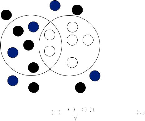
FIGURE 7.1 Venn Diagram of
Colored and Numbered Bingo Balls
|
12 |
|
6 |
4 |
|
Odd Numbers |
|
17 |
8 |
13
1
14 20
|
19 |
|
5 |
17 |
White |
|
|
2
7
12
10
18 |
16 |
ρ x, y = |
E xy − E x E y |
. |
7 4 |
|
|
||||
|
σ2 |
σ2 |
|
|
|
x |
y |
|
|
The correlation coefficient is positive, but less than one, if x and y are positively correlated. It is negative and greater than −1 if x and y are negatively correlated. If x and y are independent, then the correlation coefficient is zero.
Finally, we need to make use of Bayes’ rule. Consider Figure 7.1, which displays a Venn diagram of bingo balls that are both colored and numbered. If we consider the diagram displays the entire population of bingo balls, then there are exactly 18 balls total, with six being white and seven being odd-numbered balls. Bayes used statistical theory to determine the optimal rule for learning when combining two different pieces of information. Suppose the bingo balls in the diagram are placed in a bingo cage at the front of a large lecture hall and are drawn at random by a professor. You are seated in the back of the large lecture hall and can see the color of the ball drawn, but because you are too far away, you cannot see the number on the ball. Let us suppose that we want to know if event A = an odd numbered ball was drawn
 occurred or not. We don’t know whether A occurred and cannot observe it even if it did. But we can observe event B =
 a white ball was drawn
 , and event A and B are statistically dependent—in this case the probability of drawing an odd ball from a bingo cage containing all the balls is different from the probability of drawing an odd ball from a bingo cage containing only the white balls.
Suppose further that we have some beliefs about how likely it is that A occurred irrespective of whether B occurred. In this case, we know that seven of 18 balls are odd,
|
|
|
|
Statistical Inference and Information |
|
161 |
|
resulting in P A
A = 187 . We want to know what our observation of B tells us about A. Bayes’ rule tells us how to combine the information about underlying probabilities and the observable information about a draw to update our beliefs about the unobservable events. Let our prior beliefs regarding the probability of A be represented by P
 A
A = 187 . This function is commonly called a prior, representing the probability with which we believe A will occur if we did not have the chance to observe B. We also know that there are only two balls that are both white and odd numbered. So we know the probability of A and B occurring together is P
 A
A  B
B = 182 . Then the probability of B occurring when A has occurred is given by P
 B
B A
A , the conditional probability function, which is defined as
P B A = |
P A B |
= |
2 18 |
= 2 . |
7 5 |
P A |
|
||||
|
7 18 7 |
|
|||
In other words, the probability of B given that A has occurred is just the probability of both occurring (the fraction of times that both occur together) divided by the probability that A occurs (the fraction of times that A occurs regardless of B). This conditional probability density is often referred to as the likelihood function, and it tells us the probability of a ball being white given that it is odd numbered.
What we really want to know, however, is P A
A B
B , the probability of the ball being odd given that the ball drawn was white. Rearranging equation 7.5, we find that
P B A P A = P A B = |
2 |
. |
7 6 |
|
|||
18 |
|
|
|
The same calculations can be used to show that
P A B P B = P A B = |
2 |
. |
7 7 |
|
|||
18 |
|
|
|
By combining equations 7.6 and 7.7, we find Bayes’ rule
|
P B A P A |
2 |
7 |
|
||||
P A B = |
= |
7 |
|
|
18 |
|
||
P B |
|
|
6 |
|
|
|
||
|
|
|
|
|
|
|||
|
|
|
18 |
|
|
|||
|
|
|
|
|
|
|||
= |
1 |
. |
7 8 |
|
|||
3 |
|
|
|
Here, the value P B
B = 186 results from there being a total of six white balls. Thus, if we observe a white ball being drawn, there is a 13 probability that the ball is odd numbered.
An additional illustration of how this may be used is helpful. Suppose you knew that there were two urns full of red and white balls. Urn 1 contains 80 red balls and 20 white balls, and urn 2 contains 50 red balls and 50 white balls. Without you being able to observe, I roll a die and select an urn. If the die roll is 3 or higher, I select urn 2, and I select urn 1 otherwise. Then, I draw one ball out of the selected urn and allow you to observe its color. Suppose the ball is red. What is the probability that I have drawn from urn 1? We can rewrite equation 7.8 thus:
P Urn 1 |
Red = |
P Red Urn 1 P Urn 1 |
. |
7 9 |
|
||||
|
|
P Red |
|
|