Making Decisions for Our Future Self

The key to both the college admissions story and the example dealing with kidney disease is projection bias. Projection bias supposes that people believe they will value options in the future the way they value them today. They tend to ignore the impact of some factors that should change in the intervening time. In the case of weather and college admissions, the individual observation of weather (cloudy or sunny) has little to do with overall climate. At a university, any individual day a student chooses to engage in an activity will obtain utility uactivityuniversity, w, where activity represents the chosen activity with possible values {study recreate}, university represents the chosen university, which can take on values {prestige, party}, and w represents weather, which can take on the values {cloudy, sunny}. Suppose that at the prestigious university, recreation options are very poor but still just slightly better than studying (only a slight abstraction). Thus, on a sunny day, a student decides to recreate, receiving utility urecreateprestige, sunny, with ustudyprestige, sunny < urecreate prestige, sunny. But on a cloudy day, the student chooses to study, urecreate prestige, cloudy < ustudyprestige, cloudy.

Suppose that at another university under consideration (the party school), there are

lower than the utility for studying at the prestigious university on either sunny or cloudy days. There are spectacular opportunities to recreate at the party school, thus urecreateprestige, sunny < urecreateparty, sunny. Recreating when it is sunny is always chosen. However, when it is cloudy, despite the poor opportunities to study,

Suppose every year, exactly half of the days are cloudy and half are sunny at both schools. Thus, if the student in question decided which college to attend based upon the additive utility model, with discount factor δ = 1, we could write the utility of the

where N is the number of school days. Alternatively, at the party school the student would obtain

If ustudyprestige, cloudy − ustudyparty, cloudy < urecreateparty, sunny − urecreateprestige, sunny, then Uparty > Uprestigioius, and the student should

urecreateprestige, sunny, then the student should choose the prestigious school no matter what the weather on the day of the visit.

Suppose, however, that students ignore the impact of weather on the utility of either recreation or studying, gauging their future utility based on the state of the weather that particular day. In this case, students visiting on a cloudy day might instead perceive

but would perceive the utility of attending the party school as

In this case, they would be led to choose the prestigious university. Alternatively, if they visited on a sunny day, they would perceive

in which case they would be led to choose the party school. Though when they actually arrive on either campus they will be subject to both sunny and rainy days, they might not consider this variation when comparing the two options. Such a process could explain why students visiting on cloudy days were more likely to choose to attend the prestigious university than those visiting on sunny days. It suggests that people bias their projection of the utility of an action in the future toward the utility they assign to that action at the moment.

Notably, if people are subject to projection bias, it can create situations in which they will regret their decisions, believing that they made a mistake. In the case of this example, if ustudyprestige, cloudy − ustudyparty, cloudy < urecreateparty, sunny − urecreateprestige, sunny, students would be better off at the party school, but if they visited the campus on a cloudy day, they choose the prestigious university. At the time of the decision, they consider the utility of studying because it seems that this will be what matters. After beginning to attend, students are exposed to sunny days (about half) and might realize that the party school would be a better option. When people at one period in time believe they will have one set of preferences in the future, but then later realize systematically inconsistent preferences, we call this time-incon- sistent preferences.

George Loewenstein, Ted O’Donoghue, and Matthew Rabin proposed a model of projection bias based on the notion that people may be able to project the direction of the change in their future preferences but not the full extent of the change. In the language of the above example, they might recognize that on sunny days they will prefer to be at the party school recreating, but they might not recognize how much better off they would be at the party school on those days. Suppose that someone’s preferences can be represented by a state-dependent utility function. A person receives utility uc, s from consuming bundle c in state s. The state represents the external conditions that affect utility of consumption. This may be weather, as in Example 11.2, whether or not one has kidney

disease, as in Example 11.1, or hunger, pain, or any other factor that could influence the utility of various consumption options. Suppose someone in state s is placed in a situation where he needs to make decisions that will affect his consumption in some future state s s. In this case, the decision maker needs to predict the utility of consumption function he will face in this new state, uc, s. Let uc, ss represent the predicted utility of consumption under state s when the decision maker makes the prediction while in state s. The decision maker displays simple projection bias if

and where 0 < α ≤ 1. In this case, if α = 0, the decision maker displays no projection bias and can perfectly predict the utility of consumption he will face in the future state s. Alternatively, if α = 1, he perceives his utility in state s will be identical to his preferences in his current state s. In general, the larger the α the greater the degree of simple projection bias. Thus, the decision maker’s perception of the preferences he will realize in the future state lies somewhere between the preferences he will actually face and those that he currently holds.

People facing an intertemporal choice problem (see equation 11.1) in which the state affecting their preferences would change in the second period would thus solve

maxc1 uc1, s + δuw − c1, ss = uc1, s + δ1 − αuw − c1, s + αuw − c1, s, 1111

where 0 ≤ c1 ≤ w. A pair of potential indifference curves representing this choice when δ = 1 appear in Figure 11.2. Here, if α = 0, then they do not display projection bias, and they perceive correctly that their future utility will be maximized at point B, where the indifference curve accounting for their true future utility is tangent to the budget

c2

U = u(c1, s') + u(c2, s')

constraint. This indifference curve, represented by the dashed curve in the figure, represents the highest level of utility it is possible to achieve. Alternatively, if α = 1, then they will choose to consume at point A, where the indifference curve that assumes today’s state persists for both periods is tangent to the budget curve. Point A lies closer to the origin than the dashed curve does, meaning that people are clearly worse off when choosing point A. The points between A and B represent the different possible bundles that people might choose given different values of α. The higher the level of projection bias, α, the closer the consumption bundle will be to point A and the lower the corresponding level of utility will be realized.

Projection bias unambiguously makes people worse off than if they could perceive the true preferences they would face in the new state. It is a relatively simple way to explain a multitude of behaviors we observe in which people tend toward actions they will later regret.

Projection Bias and Addiction

One commonly regretted action is that of acquiring an addictive habit. Suppose, for example, that we consider developing a habit of drinking coffee. One key feature of an addictive habit is that as one consumes the substance, one begins to require more of it, suggesting that marginal utility is increasing. A very simplified model of this considers a decision maker in two periods. In each period, suppose that the consumer decides how much coffee to consume and how much food to consume. The consumer has an initial endowment of wealth equal to w that can be used over the two periods and receives no further income.

Let’s suppose that the consumer has an instantaneous utility function of the form

where xc, t is the consumption of coffee at time t, and xf , t is the consumption of food at time t, and where γ1, γ2 and γ3 are positive parameters with γ1 > 2. This utility function implies that the marginal utility of consuming coffee in any period (the instantaneous marginal utility) is given by

Given prior consumption, xc, t − 1, this is just a downward-sloping line with respect to current consumption, xc, t, with constant γ1 + xc, t − 1. Thus, the marginal utility of consumption increases when prior consumption, xc, t − 1, increases. However, prior consumption decreases total utility (see the third term of the utility function in equation 11.12), indicating that more consumption would be needed to obtain the same level of utility. The marginal utility of consuming food is constant

Let us suppose that before the first period, no coffee has been consumed, so that xc, 0 = 0. A consumer displaying a simple coefficient of projection bias of α (and with discount factor δ = 1) will solve

maxxc, 1, xf , 1, xc, 2, xf , 2Uxc, 1, xf , 10 + αUxc, 2, xf , 20 + 1 − αUxc, 2, xf , 2xc, 1

Projection bias in this case is associated with believing that the instantaneous utility function will not change no matter how much coffee is consumed in this period. The budget constraint must hold with equality given the positive marginal utility for drinking coffee and eating food. We can rewrite equation 11.15 as

1117

subject to equation 11.16. Because δ = 1, food will offer the same marginal utility, one, whether consumed in the first or second period. Because units of food and coffee are assumed to have the same price, the solution to equation 11.15 will occur where the marginal utility of consumption for each good in each period is equal.

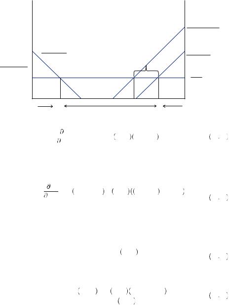
Intuitively, a consumer would always spend his next dollar on the item and period that yield the largest marginal utility. Marginal utility of coffee consumption in any period is declining with additional consumption, while the marginal utility of food consumption is constant at one. This is depicted in Figure 11.3, where the vertical axis measures marginal utility, the horizontal axis measures quantity of coffee consumption in period 1 as you move from the far left toward the right, coffee consumption in the second period is measured on the horizontal axis as you move from the far right toward the left, and food consumption is measured on the horizontal axis as the space between coffee consumption in period 1 and period 2. The consumer will choose to consume coffee in both periods until marginal perceived utility in that period declines to 1 or until the budget constraint is met. If the budget is large enough that enough coffee can be purchased in each period so that marginal utility of coffee consumption has declined to one for both periods, then the remaining money will all be spent on food.

We will assume that the budget is large enough for this to be the case. Given equation 11.15, the marginal simple projected utility of coffee consumption in the first period is given by

The consumer plans to consume the same amount of coffee in the future as he does in this period. However, when the next period comes, he instead is led to consume where instantaneous marginal utility, equation 11.13, is equal to 1, depicted in the figure as the solid marginal utility curve on the right side, or

which is satisfied if xc, 2 = γ1 − 1γ2 + xc, 1γ2. This results in an additional xc, 1γ2 > 0 of coffee he had not planned on purchasing or consuming. This requires him to cut planned food consumption by the same amount, substituting more of the addictive good for the nonaddictive good.

If instead, the consumer displays some lower degree of projection bias, equation 11.20 tells us that he will at least anticipate consuming some 1 − αxc, 1γ2 of this additional amount. But again, when he finally arrives in the second period having consumed xc, 1, he is led to consume xc, 2 = γ1 − 1γ2 + xc, 1γ2 and is forced to cut back on planned food consumption in order to do it.

In general, the simple projection-bias model predicts that people will consume more of the addictive good than they plan in future periods because they did not realize exactly how addictive the substance was. This also means they eat less food in the second period. In general, addictive behaviors crowd other consumption activities out more than the consumer anticipates. Those who become compulsive viewers of pornography don’t set out to lose their job when they become unable to resist viewing pornography at work. This misperception of the potency of addiction is the true contribution of the behavioral approach. This model of simple projection bias is procedurally rational in that it explains why people make decisions that are inconsistent with their initial plans. Rational approaches cannot explain this. Rather, models of rational addiction (proposed by Gary Becker) suppose that the preference for the addictive substance increases, but at a rate that is predictable and under the rational control of the decision maker. This appears to be inconsistent with individual experience. This is why addiction is thought of as such a pernicious trap.

Second, consider now the level of overall utility implied by consuming according to the simple projection bias model. Because consumers misperceive the level of utility they will obtain from consuming coffee in the second period, they fail to maximize their utility. The degree to which they fall short depends on α. People who can accurately project their future utility should be better off for this ability. These two results (both the reduction in utility and the tendency to increase consumption over the amount planned) are general results that should apply to all similar models of addiction with projection bias given positive instantaneous marginal utility of consumption for the addictive good.

EXAMPLE 11.3 Shopping while Hungry

Projection bias can affect consumers in profound ways. One of the clearest examples of this is found in the arena of supermarket shopping. You have probably been given the advice never to shop for food while you are hungry because you will buy more food than you need. Although this advice was originally based on folk wisdom, several behavioral

experiments verify that people do indeed purchase more food when they are hungry, and they buy foods that are more indulgent. For example, Daniel Gilbert, Michael Gill, and Timothy Wilson ran a series of experiments in which shoppers at a grocery store were stopped on their way into the store and asked to participate in a food taste sample. They were then asked to list the things they planned to buy that day at the store. One set were then given a muffin to eat before they entered the store, and others were asked to return after they finished shopping and were given a muffin afterward. As you would expect, those who had the muffin before entering the store were on average less hungry than those who were not given the muffin. Those who had to wait until after shopping to receive the muffin had to shop hungry (or at least hungrier than their counterparts). After shopping, all receipts were collected to compare actual purchases to what the shoppers had planned to buy.

In total, 111 participants took part in the experiment. Those who had eaten a muffin before shopping made many purchases that were unplanned, about 34 percent. However, more than half (51 percent) of the items purchased by those who had not eaten a muffin were unplanned. Projection bias is a likely explanation for the difference. When you are hungry, food is attractive. Each item you pass in the store may be evaluated for how it would satisfy your current hunger and you might thus decide to pick up several items that would be particularly satisfying. Alternatively, when you are not hungry, you might not consider the impact on your enjoyment of consumption at some future date when you will be hungry. In this case, many of the items that would be particularly attractive to a hungry shopper are not as immediately attractive. Thus, they buy fewer of the items they had not planned on purchasing.

A potentially more convincing experiment was conducted by Daniel Read and Barbara van Leeuwen. People were asked in their place of work to choose a snack that they would receive in exactly one week. Some of the snacks were relatively healthy choices, and others would be considered indulgent. Some participants were told they would receive the snack in the late afternoon, and others were told they would receive the snack immediately after their lunch break. Those receiving the snack in the afternoon would anticipate that they would be hungry in the future. Those receiving the snack right after lunch would expect not to be hungry. Additionally, some participants were asked this question right after lunch, and others were asked late in the afternoon. Table 11.1 displays the percentage of participants who chose indulgent snacks in each of the four conditions. As can be seen, people who were hungry were more likely to choose indulgent snacks than those who were not hungry, and those who were choosing for a future hungry state were more likely to choose the indulgent snacks.

Table 11.1 Percentage Choosing Unhealthy Snacks by Current and Future

Level of Hunger

Source: Read, D., and B. van Leeuwen. “Predicting Hunger: The Effects of Appetite and Delay on Choice.”

Organizational Behavior and Human Decision Processes 76(1998): 189–205.

Let ch represent consumption of healthy snacks, and let ci represent consumption of indulgent snacks. Further, let sh represent a state of hunger, and sn represent not being hungry. Let uc, s be the utility of consuming c while experiencing hunger state s. Suppose first that people find indulgent treats more attractive when they are hungry, uci, sh > uci , sn and that healthy snacks are less attractive, uch, sh < uch, sn. Finally, let us suppose that indulgent food is preferred when people are hungry, uch, sh < uci , sh, and healthy food is preferred when people are not hungry, uch, sn > uci , sn. Consider someone who suffers from simple projection bias. In a hungry state, considering his future consumption in a hungry state, he will consider

and choose the indulgent snack. In this case he displays no projection bias and correctly chooses the indulgent snack in the future (78 percent chose this). Alternatively, if he is not hungry and is choosing his future consumption in a state in which he is not hungry, he will consider

and choose the healthy snack. In this case, he again displays no projection bias and correctly chooses the healthy snack for his future self (74 percent chose this).

The problem only arises when one is choosing for a future hunger state that is different. A hungry person considering his consumption in a future state when he is not hungry will consider his projected utility of consuming the healthy snack

versus the projected utility of consuming the indulgent snack

Which is larger critically depends critically on the degree of projection bias, α. If α = 1, perfect projection bias, then the person will choose the indulgent outcome, behaving as if he will be hungry in the future. Of the participants, 42 percent chose this option, much more than those who were not hungry. If α = 0, the person would choose the healthy item. We observe that 38 percent of participants chose this option, many fewer than chose the healthy option when they are not hungry.

The data in Table 11.1 are consistent with the notion that at least some people display a high enough degree of projection bias that they will choose something for their future self that they would not want. The projection bias distorts their perception of the value of the tradeoffs involved in the choice. If this model of choice is right, people choosing for future states that are similar to today will be much better off than those choosing for different states. This brings us back to the question of whether to shop when you are hungry.

Certainly we have evidence that shopping for food while hungry will increase the number of purchases and likely decrease the nutritional content. However, if you intend to eat the food at some future time when you are hungry, this might make you better off

in the end. The advice given by this behavioral model is to shop when in a hunger state that is similar to that in which you will choose to consume the food. The difficulty with this notion arises when the presence of indulgent food might affect how one assesses one’s hunger, or if simply having the indulgent food leads one to eat whether it is the preferred food or not. The advice to only shop on a full stomach makes sense only if one is trying to impose some less-preferred behavior on one’s future self. For example, a person might want to stay within a budget or be trying to lose weight. He knows if he shops in a hungry state he will purchase more or will purchase foods that when consumed will make him fat.

EXAMPLE 11.4 Impulse Buying and Catalogue Purchases

In the depths of winter, a vacation to the Caribbean may be very attractive. However, if you are planning for a vacation to be taken in August, it may be hard to remember that you will be leaving the August frying pan of your hometown for the August fire of the Caribbean. In the end it may be an unpleasant trip.

Simple projection bias suggests that weather might actually affect many of our decisions about future consumption. Consider ordering clothes out of a catalogue. When perusing a catalogue on a particularly cold day, your body’s desire for warmth can color the projected enjoyment you will obtain from warmer clothing. On the other hand, when you receive the item, you might not be subject to the same projection bias any longer and simply decide to return it.

Michael Conlin, Ted O’Donoghue, and Timothy J. Vogelsang obtained records of more than 2 million catalogue sales of gloves, mittens, boots, hats, winter sports equipment, parkas, coats, vests, jackets, and rainwear. Each was an item that would be particularly useful in cold, snowy, or rainy weather—but not much use otherwise. Using regression analysis, they found that people are more likely to return the cold-weather items if the weather was particularly cold when they purchased them. In particular, if the temperature is 30 degrees cooler on the date of purchase, buyers are 4 percent more likely to return the item once they receive it. Similarly, more snowfall on the date of purchase leads to a higher probability of return. Both of these could also be explained potentially by people just being more inclined to purchase frivolously on cold or snowy days (i.e., I am stuck inside because of the weather so I buy clothes through a catalogue as entertainment). This led them to see if people would return more of the items they purchase during cold weather even if those items were not related to cold weather (e.g., windbreakers). When conducting similar analysis of nonwinter coats and gear they found no similar relationship, suggesting that projection bias, rather than boredom, is driving the frivolous purchases of later unwanted items.

If projection bias is driving the purchases of these cold-weather items, you would also expect that people would display some amount of projection bias at the time they decide whether or not to return the item. Once I have received my cold weather gear, if it is relatively cold over the period in which I can return the item, I may be less likely to return it. This relationship is not as easily seen in Conlin, O’Donoghue, and Vogelsang’s analysis, partially because it is impossible to know the date the buyer makes this