
- •Brief Contents
- •Contents
- •Preface
- •Who Should Use this Book
- •Philosophy
- •A Short Word on Experiments
- •Acknowledgments
- •Rational Choice Theory and Rational Modeling
- •Rationality and Demand Curves
- •Bounded Rationality and Model Types
- •References
- •Rational Choice with Fixed and Marginal Costs
- •Fixed versus Sunk Costs
- •The Sunk Cost Fallacy
- •Theory and Reactions to Sunk Cost
- •History and Notes
- •Rational Explanations for the Sunk Cost Fallacy
- •Transaction Utility and Flat-Rate Bias
- •Procedural Explanations for Flat-Rate Bias
- •Rational Explanations for Flat-Rate Bias
- •History and Notes
- •Theory and Reference-Dependent Preferences
- •Rational Choice with Income from Varying Sources
- •The Theory of Mental Accounting
- •Budgeting and Consumption Bundles
- •Accounts, Integrating, or Segregating
- •Payment Decoupling, Prepurchase, and Credit Card Purchases
- •Investments and Opening and Closing Accounts
- •Reference Points and Indifference Curves
- •Rational Choice, Temptation and Gifts versus Cash
- •Budgets, Accounts, Temptation, and Gifts
- •Rational Choice over Time
- •References
- •Rational Choice and Default Options
- •Rational Explanations of the Status Quo Bias
- •History and Notes
- •Reference Points, Indifference Curves, and the Consumer Problem
- •An Evolutionary Explanation for Loss Aversion
- •Rational Choice and Getting and Giving Up Goods
- •Loss Aversion and the Endowment Effect
- •Rational Explanations for the Endowment Effect
- •History and Notes
- •Thought Questions
- •Rational Bidding in Auctions
- •Procedural Explanations for Overbidding
- •Levels of Rationality
- •Bidding Heuristics and Transparency
- •Rational Bidding under Dutch and First-Price Auctions
- •History and Notes
- •Rational Prices in English, Dutch, and First-Price Auctions
- •Auction with Uncertainty
- •Rational Bidding under Uncertainty
- •History and Notes
- •References
- •Multiple Rational Choice with Certainty and Uncertainty
- •The Portfolio Problem
- •Narrow versus Broad Bracketing
- •Bracketing the Portfolio Problem
- •More than the Sum of Its Parts
- •The Utility Function and Risk Aversion
- •Bracketing and Variety
- •Rational Bracketing for Variety
- •Changing Preferences, Adding Up, and Choice Bracketing
- •Addiction and Melioration
- •Narrow Bracketing and Motivation
- •Behavioral Bracketing
- •History and Notes
- •Rational Explanations for Bracketing Behavior
- •Statistical Inference and Information
- •Calibration Exercises
- •Representativeness
- •Conjunction Bias
- •The Law of Small Numbers
- •Conservatism versus Representativeness
- •Availability Heuristic
- •Bias, Bigotry, and Availability
- •History and Notes
- •References
- •Rational Information Search
- •Risk Aversion and Production
- •Self-Serving Bias
- •Is Bad Information Bad?
- •History and Notes
- •Thought Questions
- •Rational Decision under Risk
- •Independence and Rational Decision under Risk
- •Allowing Violations of Independence
- •The Shape of Indifference Curves
- •Evidence on the Shape of Probability Weights
- •Probability Weights without Preferences for the Inferior
- •History and Notes
- •Thought Questions
- •Risk Aversion, Risk Loving, and Loss Aversion
- •Prospect Theory
- •Prospect Theory and Indifference Curves
- •Does Prospect Theory Solve the Whole Problem?
- •Prospect Theory and Risk Aversion in Small Gambles
- •History and Notes
- •References
- •The Standard Models of Intertemporal Choice
- •Making Decisions for Our Future Self
- •Projection Bias and Addiction
- •The Role of Emotions and Visceral Factors in Choice
- •Modeling the Hot–Cold Empathy Gap
- •Hindsight Bias and the Curse of Knowledge
- •History and Notes
- •Thought Questions
- •The Fully Additive Model
- •Discounting in Continuous Time
- •Why Would Discounting Be Stable?
- •Naïve Hyperbolic Discounting
- •Naïve Quasi-Hyperbolic Discounting
- •The Common Difference Effect
- •The Absolute Magnitude Effect
- •History and Notes
- •References
- •Rationality and the Possibility of Committing
- •Commitment under Time Inconsistency
- •Choosing When to Do It
- •Of Sophisticates and Naïfs
- •Uncommitting
- •History and Notes
- •Thought Questions
- •Rationality and Altruism
- •Public Goods Provision and Altruistic Behavior
- •History and Notes
- •Thought Questions
- •Inequity Aversion
- •Holding Firms Accountable in a Competitive Marketplace
- •Fairness
- •Kindness Functions
- •Psychological Games
- •History and Notes
- •References
- •Of Trust and Trustworthiness
- •Trust in the Marketplace
- •Trust and Distrust
- •Reciprocity
- •History and Notes
- •References
- •Glossary
- •Index

|
|
|
|
|
116 |
|
THE WINNER’S CURSE AND AUCTION BEHAVIOR |
between the laboratory outcomes and the real-world outcomes. In essence, they found three real reasons why the winner’s curse is rare in construction bidding.
First, contractors monitor the difference between their bid and the bids of others on any particular project. They monitor closely enough that they have a good feel for the average difference between the top and second bid for various types of jobs. When the differences between the lowest (winning) and the next lowest bid were greater than about 7 percent, they often inquired of other bidders to determine the reason for the difference, a clear sign that they were aware of and worried about the winner’s curse. Contractors also clearly understand the need to mark up bids in anticipation of random costs that might occur unforeseen in the construction process.
The second mechanism that allows a contractor to avoid the winner’s curse is the ability to withdraw an apparent winning bid once all bids have been announced if there has been any arithmetic error in calculating the bid. In this case, winning the bid with a significant distance between the top and second bid might lead a contractor to reevaluate the bid and search for reasons for the difference. If the difference is due to an error, he may withdraw the bid.
Finally, the contractor has the ability to adjust costs. For example, in the course of construction some of the plans might change, allowing the bidder to renegotiate for higher pay in midstream. The lesson from this study appears to be that the winner’s curse is a real threat, but industries with experience in bidding might find heuristics and other mechanisms to reduce or eliminate the threat.
History and Notes
The term winner’s curse was first coined by Capen, Clapp, and Campbell in their description of the oil lease contracts of the 1950s and 1960s. The early study of the winner’s curse was driven first by field data from various industries. The notion has become quite popular in describing many different phenomena where parallels can be drawn. The winner’s curse has inspired research-based books by Richard Thaler and by John Kagel and Dan Levin and a score of popular books by various authors. For participants in bidding, the implication is clear. One must scrutinize one’s bid with the goal that the bid should likely be below the lowest possible value one would consider for the good. This is especially important when there are large numbers of bidders or when the person formulating the bid is inexperienced. Although this might result in losing the auction even when it might have been profitable, this is a much better outcome than winning the auction when it is unprofitable. From the point of view of sellers, it may be better to employ auctions with large numbers of inexperienced bidders, because this is the most likely way to generate bids well in excess of the true value of the object being auctioned.

|
|
|
|
Rational Explanations for the Winner’s Curse |
|
117 |
|
Rational Explanations for the Winner’s Curse
Most of the rational explanations for the winner’s curse deal with identifying imperfections in the field data used to demonstrate the effect. Unfortunately, it is not generally possible to observe individual information about the value of an object in a field setting. As well, it is impossible to determine the expected profit for an object or endeavor with any degree of accuracy.
For example, in studying the oil lease contracts, it is necessary to assume specific discount factors for future consumption in order to determine if the net present value of returns is negative or positive. Assuming less discounting for the future provides a larger return. Further, there were tremendous increases in the price of oil over the period generally studied that are unlikely to have been anticipated. Similarly, estimating the overpayment of baseball players relies heavily on the underlying assumptions of that player’s value. Certainly there may be factors other than slugging, strikeouts, and walks. Finally, risk aversion alters the optimal bid and generally leads to higher bids. Thus, if winning bidders are risk averse, we would expect them to display profits that are below the expected payoutmaximizing amount on average, though these profits should not be negative on average.
All of these factors make it difficult to say with certainty that the winner’s curse has been observed in the wild. Thus, many have suggested that the winner’s curse is simply an illusion. However, this phenomenon appears to have had tremendous impacts on the way several industries respond to unknown values. The simple presence of mechanisms such as those found in the construction industry is tangible evidence that people develop heuristics to deal with the problem of the winner’s curse, while not fully understanding the mathematics behind the problem itself. These heuristics develop out of systematic experience, providing a key point of evidence that the curse exists in some contexts and is strong enough to lead to long-term changes in institutions.
Biographical Note
© KENDRA LUCK/San Francisco Chronicle/Corbis
Matthew Rabin (1963–)
B.A., University of Wisconsin at Madison, 1984; Ph.D., Massachusetts Institute of Technology, 1989; held faculty positions at the University of California at Berkeley
Matthew Rabin conducted his undergraduate study in economics and mathematics. His training has led to an approach that is behavioral, yet based on rigorous mathematical modeling of the underlying phenomena. Much of this work employs behavioral concepts in a game-theory setting. His earliest work
posits that people consider the motivations of others when deciding how to behave. For example, one might wish to help someone who has been nice to one in the past

|
|
|
|
|
118 |
|
THE WINNER’S CURSE AND AUCTION BEHAVIOR |
and might wish to harm those who have harmed one in the past. His works have contributed to behavioral theory of auctions, risk and uncertainty, the impacts of cheap talk (nonbinding talks) in games, the discounting and anticipation of future events, probability judgment bias, and welfare analysis. His colleagues describe him as a voracious reader, approaching new research by first pulling all related literature from any discipline that may be connected to it. In 2001, he won the John Bates Clark Medal, which is generally awarded to the economist younger than 40 years who has contributed the most to the field. He has won the MacArthur fellowship (often called the “Genius” fellowship). Personally, Matthew Rabin is known as an engaging teacher and presenter, endowed with more than his fair share of humor. As an example of the humor inherent in his personality, his personal résumé lists his first professional honor as being voted “Most Likely to Express His Opinion,” by the Springbrook High School class of 1981.
T H O U G H T Q U E S T I O N S
1.Consider that you are preparing to sell some antique items at auction. How might you design the auction so as to receive the highest possible sale price? What sorts of behavioral anomalies will be important to consider? What role will the number and experience of the bidders play in the auction?
2.Consider now that you are preparing to purchase an item at auction for your personal use. What factors should you consider in forming your bid? What behavioral tendencies should you try to avoid? What if you were purchasing the item for resale at a later date instead?
3.Building contractors bidding on a building project often calculate their anticipated costs, add some percentage for profit, and then double this number and submit it as a bid. Similar rules of thumb have been reported in other auction arenas. Why do you think such rules of thumb developed? What purpose do they serve? In what ways might the contractors be worse off for using this rule of thumb?
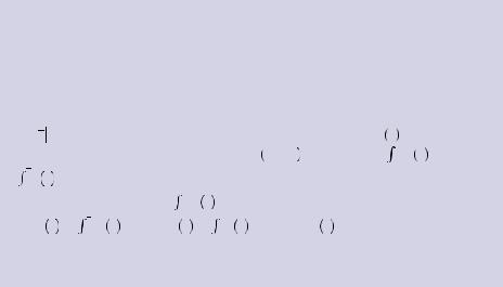
4.Suppose that two people are engaged in a Vickrey auction for a good with two possible values: $10 or $20. Further, suppose each bidder receives a signal of the value, xn, where xn is equal to the true value with probability 0.8, and equal to the other possible value with probability 0.2. No information other than this signal is available. Each player must select a bid based on his own signal. What bidding strategy would be
suggested by the fully cursed equilibrium (e.g., what should you bid if you receive a signal of $10 and what should you bid if you receive a signal of $20)? Suppose that players can only bid integer amounts, and follow the example given in the text. Thus, if player 1 draws x1 = 10, the mean value of winning the auction is μ = 0.8 × 10 + 0.2 × 20 = 12, the probability of signals that player 2 might receive is (similar to equation 5.14)
p x2 |
= 0.8 × 0.8 + 0.2 × 0.2 = 0.68 |
if |
x2 = 10 |
|
0.8 × 0.2 + 0.2 × 0.8 = 0.32 |
if |
x2 = 20. |
If player 1 draws x1 = 20, the expected value of winning the auction is μ = 0.8 × 20 + 0.2 × 10 = 18, and the probability distribution of signals that player 2 might receive is
p x2 |
= 0.8 × 0.8 + 0.2 × 0.2 = 0.68 |
if |
x2 = 20 |
|
0.8 × 0.2 + 0.2 × 0.8 = 0.32 |
if |
x2 = 10 |
Suppose that in the event of a tie, both players receive the value of the object. First try the strategy in which each player bids the expected value of the gamble given the signal each has received. Show that this constitutes a cursed equilibrium. What is the expected profit in this case (the actual, not perceived)? Do these strategies constitute a Bayesian Nash equilibrium? If not, can you find the Bayesian Nash equilibrium?
|
|
|
|
References |
|
119 |
|
R E F E R E N C E S
Ariely, D., A. Ockenfels, and A.E. Roth. “An Experimental Analysis of Ending Rules in Internet Auctions.” RAND Journal of Economics 36(2005): 890–907.
Baraji, P., and A. Hortaçsu. “The Winner’s Curse, Reserve Prices and Endogenous Entry: Empirical Insights from eBay Auctions.”
RAND Journal of Economics 34(2003): 329–355.
Capen, E.C., R.V. Clapp, and W.M. Campbell. “Competitive Bidding in High-Risk Situations.” Journal of Petroleum Technology
23(1971): 641–653.
Cassing, J., and R.W. Douglas. “Implications of the Auction Mechanism in Baseball’s Free Agent Draft.” Southern Economic Journal 47(1980): 110–121.
Cox, J.C., B. Roberson, and V.L. Smith. “Theory and Behavior of Single Object Auctions.” Research in Experimental Economics
2(1982): 1–43.
Dyer, D., and J.H. Kagel. “Bidding in Common Value Auctions: How the Commercial Construction Industry Corrects for the Winner’s Curse.” Management Science 42(1996): 1437–1475.
Eyster, E., and M. Rabin. “Cursed Equilibrium.” Econometrica
73(2005): 1623–1672.
Kagel, J.H., R.M. Harstad, and D. Levin. “Information Impact and Allocation Rules in Auctions with Affiliated Private Values: A Laboratory Study.” Econometrica 55(1987): 1275–1304.
Kagel, J.H., and D. Levin. “The Winner’s Curse and Public Information in Common Value Auctions.” American Economic Review
76(1986): 894–920.
Kagel, J.H., and J.-F. Richard. “Super-Experienced Bidders in FirstPrice Common Value Auctions: Rules of Thumb, Nash Equilibrium Bidding, and the Winner’s Curse.” Review of Economics and Statistics 83(2001): 408–419.
Lucking-Reiley, D. “Using Field Experiments to Test Equivalence between Auction Formats: Magic on the Internet.” American Economic Review 89(1999): 1063–1080.
Mead, W.J., A. Moseidjord, and P.E. Sorensen. “The Rate of Return Earned by Lessees under Cash Bonus Bidding of OCS Oil and Gas Leases.” Energy Journal 4(1983): 37–52.
Roth, A.E., and A. Ockenfels. “Last-Minute Bidding and the Rules for Ending Second Price Auctions: Evidence from eBay and Amazon Auctions on the Internet.” American Economic Review
92(2002): 1093–1103.
Samuelson, W.F., and M.H. Bazerman. “The Winner’s Curse in Bilateral Negotiations.” Research in Experimental Economics
3(1985): 105–137.
Stahl, D.O., and P.W. Wilson. “On Players’ Models of Other Players: Theory and Experimental Evidence.” Games and Economic Behavior 10(1995): 218–254.
Wilson, R. “A Bidding Model of Perfect Competition.” Review of Economic Studies 44(1977): 511–518.
Advanced Concept
Bayesian Nash Equilibrium and Bidding under Uncertainty
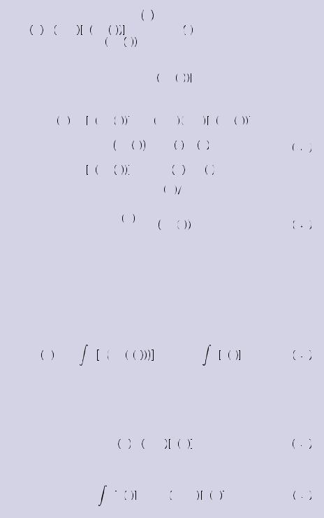
When dealing with a continuum of possible valuations, we use a probability density function to represent the likelihood of any particular draw falling in any particular range of values. Let z be a random variable with support given by
z, |
z |
. Then, the probability density function is a function f |
z such that the |
probability of z falling in any interval z1, z2 is given by |
z2 f z dz. Thus, |
||
|
|
|
z1 |
z f z dz = 1, and if the probability density is continuous, the probability of any |
|||
z |
|
|
|
single outcome is given by |
z1 f z dz = 0. We now define the expectation function |
||
|
|
z1 |
|
as E z = |
z zf z dz. Let F z = |
z f z dz. Thus, F z is the probability of any |
|
|
z |
|
z |
particular draw from the distribution falling below z. In this context, given a probability density g v
v of valuations, if the bidder believes others will bid
|
|
|
|
|
|
|
|
|
|
|
|
|
|
|
|
|
|
|
|
|
120 |
|
THE WINNER’S CURSE AND AUCTION BEHAVIOR |
|
|
|
|
|
|||||||||||
|
|
|
according to the bid function xj = b vj , his expected payoff for bidding x is given |
||||||||||||||||
|
|
|
by E πi = vi − x G b − 1 x |
n − 1. Here, b − 1 |
x is the valuation that will result |
||||||||||||||
|
|
|
in a bid of x. Hence, G b − 1 |
x is the probability of a single draw from the |
|||||||||||||||
|
|
|
distribution of valuations falling below the valuation that would bid x. To find the |
||||||||||||||||
|
|
|
probability that all other players bid less than x, we need only multiply this |
||||||||||||||||
|
|
|
probability together n − 1, times, or |
G b − 1 x |
|
n − 1. This is thus the probability |
|||||||||||||
|
|
|
of wining the auction given a bid of x. If we differentiate the expected payout with |
||||||||||||||||
|
|
|
respect to vi, we obtain |
|
|
|
|
|
|
|
|
|
|
|
|||||
|
|
|
|
d |
E πi = G b − 1 x |
n − 1 − vi − x n − 1 G b − 1 x |
n − 2 |
||||||||||||
|
|
|
|
|
|
||||||||||||||
|
|
|
dvi |
|
|
|
|
|
|
|
|
|
|
|
|||||
|
|
|
|
|
× |
d |
G b − 1 x |
d |
b − 1 x |
dx |
|
vi |
5 A |
||||||
|
|
|
|
|
|
|
|
|
|
||||||||||
|
|
|
|
|
dv |
|
|
dx |
dv |
|
|||||||||
|
|
|
|
|
= G b − 1 x |
n − 1 + |
d |
E πi |
|
d |
b x . |
|
|||||||
|
|
|
|
|
|
|
|
||||||||||||
|
|
|
|
|
|
|
|
|
|
|
|
dx |
|
dvi |
|
||||
|
|
|
When evaluated at the optimal bid, dE πi dx = 0 so that the second term of |
||||||||||||||||
|
|
|
equation 5.A is zero. Thus, |
|
|
|
|
|
|
|
|
|
|
|
|||||
|
|
|
|
|
|
|
|
dE πi |
= G b − 1 x |
|
|
n − 1, |
5 B |
||||||
|
|
|
|
|
|
|
|
|
|
||||||||||
|
|
|
|
|
|
|
|
dvi |
|
|
|
|
|
|
|
|
|
||
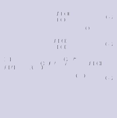
in Nash equilibrium. Further, note that no bidder should ever bid lower than the lowest possible valuation. Each bidder knows that all other bidders have a minimum valuation of v, and that bidding below this value will ensure losing the auction. Further, no one will ever bid above their valuation. Thus, we know that whatever the optimal rule, the bidder who has drawn the lowest possible valuation must bid his own valuation, b v
v = v. We can then solve for the optimal bidding strategy by solving the differential equation given by equation 5.B and the condition that b
 v
v = v. Solving equation 5.B obtains
vi |
G b − 1 x v n − 1dv = k + |
vi |
|
E πi = k + |
G v n − 1dv, |
5 C |
|
v |
|
v |
|
where k is an arbitrary constant and the second equality holds by assuming that x v
v = b
= b v
v ; in other words, all bidders with the same value make the same bid. The definition of the expected payout function (assuming again that all bidders with the same valuation submit the same bid) is given by
E πi = vi − x G vi n − 1, |
5 D |
or substituting equation 5.C we find
|
vi |
|
k + |
G v n − 1dv = vi − x* G vi n − 1. |
5 E |
v
|
|
|
|
References |
|
121 |
|
Solving equation 5.E for the optimal bid yields
|
k + |
vi |
G v |
n − 1 |
dv |
|
|
|||||
x* = vi − |
v |
|
|
|
. |
5 F |
||||||
|
|
|
|
|
|
|
|
|
||||
|
|
|
|
|
|
|
|
|
|
|||
|
|
G vi |
n − |
1 |
|
|
|
|||||
|
|
|
|
|
|
|
|
|||||
The condition requiring the lowest valuation to result in b v |
= v allows us to |
|||||||||||
solve for the constant, k = 0. Hence, the optimal bid is given by |
||||||||||||
|
|
vi |
G v |
n − 1 |
dv |
|
|
|||||
x* = vi − |
v |
|
|
|
|
|
||||||
|
|
|
|
|
|
|
. |
|
5 G |
|||
|
G vi |
n − |
1 |
|
|
|
||||||
|
|
|
|
|
|
|
|
|||||
In the special case when the distribution of v is uniformly distributed on support
0, |
|
, the probability density is given by g v |
= 1 v over the support and zero |
|||||||||||||||||||||||
v |
||||||||||||||||||||||||||
|
|
|
|
|
|
|
|
|
|
= |
v |
|
|
|
|
|
|
|
|
|
vi |
|
n − 1 |
|
||
elsewhere. |
Thus, |
|
G v |
1 |
vdv = v v. |
|
Also, |
G v |
dv = |
|||||||||||||||||
|
0 |
|
0 |
|
||||||||||||||||||||||
0vi v |
|
n − |
1dv = vin |
|
|
|
|
|
|
|
|
|
|
|
|
|
|
|
|
|
|
|
||||
|
|
n − 1n . Thus, |
|
|
|
|
|
|
|
|
|
|
|
|
||||||||||||
v |
v |
|
|
|
|
|
|
|
|
|
|
|
|
|||||||||||||
|
|
|
|
|
|
|
|
|
|
|
|
n − 1vin |
|
|
|
vi |
|
|
n − 1 |
|
|
|
|
|||
|
|
|
|
|
x* = vi − |
|
|
v |
|
|
= vi − |
= vi |
, |
|
|
5 H |
||||||||||
|
|
|
|
|
|
|
|
n − 1vn − 1 |
n |
|
n |
|
|
|||||||||||||
|
|
|
|
|
|
|
nv |
|
|
|
|
|
|
|
||||||||||||
|
|
|
|
|
|
|
|
|
|
|
|
|
|
i |
|
|
|
|
|
|
|
|
|
|
|
|
which is the result reported in equation 5.9. When we employ a Nash equilibrium in a game of uncertainty such as this we refer to it as a Bayesian Nash equilibrium. This is in reference to the requirement that each player must have beliefs regarding the strategies and payoffs of all other players that is consistent with their strategies in the equilibrium. Thus, in this game we require that each player has the same prior beliefs regarding the distribution of valuations and that each anticipates the correct strategy of others given their valuation.
INFORMATION AND UNCERTAINTY
PART2
Many decisions involve outcomes that are unknown at the time of making a decision. For example, homebuyers may opt to purchase flood or earthquake insurance but must decide to do so before it becomes obvious whether or not a flood or earthquake will inflict damage on their home. Investment, education, family planning, production, and other decisions all require decision makers to leap before they can look. Economics has proposed a welldeveloped and intuitively satisfying theory for how people make decisions when facing uncertainty; this theory is built on the work of John von Neumann and Oscar Morgenstern in proposing a rational decision framework.
However, there has been evidence from early on of behavioral anomalies in decision under risk. Such decisions are particularly prone to behavioral anomalies because of the random nature of the outcomes. For example, consider the case where a homebuyer insures her house against flooding when it would be in her best interest not to. Perhaps she overestimated the relative frequency of floods. In other words, given her tolerance for risk, she would be better off not purchasing insurance and facing the risk of catastrophic loss from a flood given the relative rarity of flooding near her home. Given that flooding is relatively rare, she might not particularly notice or revise her beliefs regarding the frequency of floods over the course of many years without an observed flood.
With any event that happens with relative rarity, people can have a very hard time distinguishing between events with vastly different relative frequency. Behavioral economists have noted several behavioral anomalies that are relatively predictable, and they have proposed alternative theories as to why these anomalies occur. This section of the book presents many of these theories, which can be divided into three general categories: theories of learning, theories of decision under uncertainty, and choice bracketing. I begin with choice bracketing because it makes a relatively easy transition from consumer theories to the theory of decision under risk.
123

Bracketing Decisions
6
Consider your friend who has a final paper due in a relatively important class. The paper will be worth about half of his grade in the class. It is Friday at 7:00 P.M., and he must complete the paper by Monday morning at 9:00 A.M. He believes that the paper will take about six hours of hard work to complete. However, he is in the middle of a role-playing video game and is really itching to play the game for at least another 20 minutes before diving into his paper. Upon considering his options, he believes the 20 minutes will not set him back too far because it is such a small amount of time. Further, the 20 minutes would not allow him to make very much progress at all on his paper relative to the amount of progress he might be able to make on the game. Thus, he decides to play. About 20 minutes later, he faces the same decision. But 20 minutes still seems like such a short period compared to the amount of time he has left to finish the paper. So, he continues to play. At about 3:00 A.M., after playing for eight hours, he decides to go to bed and work on the paper the next day. He regrets the amount of time he spent playing video games, and realizes that he could have made significant progress on the paper and could perhaps have completed it by then. He laments, “How could I have played video games for eight hours instead of working on my paper?”
Consider, alternatively, a company headed by two people: a CEO and a president of operations. The CEO has ultimate responsibility for the company, and the president directly oversees the eight team leaders who make up the senior management. Each of the team leaders has some autonomy and can decide on the particular projects that they will undertake. The CEO is worried that although the company is profitable, profits are smaller than she would like. Wondering the root cause of the problem, she calls on the president to consider the problem. The president meets one by one with each team leader, asking for detailed accounts of their decision-making process. He finds that each has engaged in relatively safe projects. As well, each has turned down some risky projects. For example, a typical risky project would return $20 million with about 50 percent probability and lose $10 million with 50 percent probability. Considering the overall budget of this individual team is only around $20 million, the president considers the decision to scuttle such risky projects sound. He compiles his report detailing the similar decision processes and abandoned opportunities from each of the eight teams to the CEO. The CEO, upon reading about the potential for eight projects, each returning about $20 million with 50 percent probability, and losing $10 million with 50 percent probability, calculates the expected value to be $40 million, with less than a 15 percent chance of losing any money. She immediately fires the president of the company.
125
