


 . Thus, the choice between
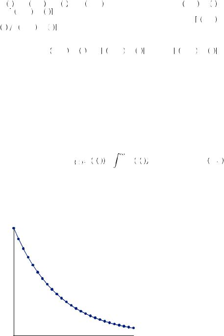
 that indicates planned consumption at each point in time. Figure 12.2 displays the discount applied over time
|
|
|
|
Why Would Discounting Be Stable? |
|
313 |
|
the dashed line displays the discount factor for a continuous-time model. The exponential discounting model discounts instantaneous utility according to the standard exponential function, creating the familiar function that slopes down and to the right. Asymptotically, as time stretches to infinity, the discount factor converges to zero. Thus, the model implies that people care less and less about the future the farther into the future we consider.
At first blush, it might seem arbitrary to assume that every period receives an identical discount, δ. There are two primary motivations for this assumption. First, it would be difficult to analyze models with discount factors that change over time. Manipulating models representing a general case where discounting can differ in every period would only be possible to analyze using sophisticated computer programs, and it would yield very few general or intuitive results. For this reason, assuming a stable discount factor from period to period became common early in economic work examining intertemporal choice. Additionally, Robert H. Strotz noted that a constant discount factor was required if people are to display time-consistent preferences.
Why Would Discounting Be Stable?
Because the mathematics of multiperiod intertemporal choice problems can get very complicated, it can often be useful to consider a very simplified version of the model. For example, suppose that a person had to choose between two consumption profiles. The first of the available consumption profiles would offer c1 = 20 in the first period, c2 = 19 in the second period and, c3 = 18 in the third period, which we will write c =  20, 19, 18
 . The second of these options offers c′ =
 20, 18, 19
 . Once a consumption profile is chosen, the person is not allowed to change her choice in later periods even if she wishes to do so. We would not expect this restriction to be a problem to rational people if they can predict their own preferences in the future. Choosing one consumption profile in the first period and then wishing one had chosen the other once the second period is reached would result in time-inconsistent preferences. Notably, consumption in both profiles is equal in the first period, so it is really only consumption in later periods that matters when making the decision.
Suppose that the person discounts utility of consumption in the next period (tomorrow) by δ2 and discounts utility two periods from now (the day after tomorrow) by δ3. These discount factors allow the decision maker to discount at different rates depending on how far into the future the decision is, but she always treats tomorrow the same, and she always treats the day after tomorrow the same. Thus, in the first period the decision
maker will choose c if |
|
u 20 + δ2u 19 + δ3u 17 > u 20 + δ2u 18 + δ3u 19 . |
12 4 |
Subtracting u 20
20 from both sides of this inequality and collecting terms, this can be rewritten as
δ2 > δ3 |
u 19 |
− u 17 |
. |
12 5 |
u 19 |
|
|||
|
− u 18 |
|
||

|
|
|
|
|
314 |
|
NAÏVE PROCRASTINATION |
Suppose that this is the case, and that the person chooses c. She will consume 20 in the first period and then enter the second period committed to the remainder of her consumption profile cR = 19, 178
 , having passed up the remainder of the consumption profile cR ′ =
 18, 19
 . However, now the person judges period 2 as the current period and applies no discount to second-period consumption. As well, period 3 is now the next period and will be discounted by δ2, rather than δ3, as it was previously. If she had been able to choose which of these consumption profiles to pursue in period 2, she would have chosen cR if
u 19 + δ2u 17 > u 18 + δ2u 19 |
12 6 |
|||
or |
|
|
|
|
δ2 |
< u 18 |
− u 19 |
, |
12 7 |
|
u 17 |
− u 19 |
|
|
where the inequality flips because u 17
17 − u
− u 19
19 < 0. If equation 12.7 holds, the person would regret having chosen c. Whether both equations 12.5 and 12.7 can be satisfied depends upon the values of δ3, δ2 and the instantaneous utility functional form.
For example, suppose that u ci
ci =
= ci, and let δ2 = 0.45, with δ3 = 0.45λ. If we evaluate the choice from the point of view of the consumer in the second period, equation 12.7 can be rewritten as
δ2 = 0.45 < |
4.24 |
− 4.36 |
0.5, |
12 8 |
|
4.12 |
− 4.36 |
|
|
meaning that because δ2 < 0.5, the person will always prefer consumption profile cR once the second period is reached. However, if we evaluate the choice from the point of view of a first-period consumer, equation 12.5 can be rewritten as
δ3 |
u 19 |
− u 17 |
= 0.45λ |
4.36 |
− 4.12 |
λ0.9 < 0.45 = δ2. |
12 9 |
|
u 19 |
− u 18 |
4.36 |
− 4.24 |
|||||
|
|
|
|
Thus, in the first period, the person would commit to the consumption profile c only if
λ< 0.5. In the case of constant discounting, λ = δ2 = 0.45, in which case the person would prefer c in the first period and also once the second is reached. However, if λ > 0.5, then the person would commit to c′ in the first period, but once the second period was
reached she would regret her actions and wish she had chosen c. In this case, a value of
λ> 0.5 generates time-inconsistent preferences.
Though consumption under both choices is identical in the first period, under λ > 0.5 the decision maker in the first period believes she will be patient enough once she enters the second period to be willing to trade off consumption of one unit in the second period to obtain two additional units in the third. However, once the person enters the second period she finds that her preferences are different from what she anticipated. Instead, she would prefer the additional unit of consumption now than to wait until the third period to consume two additional units.
|
|
|
|
|
|
|
|
|
|
|
|
|
|
|
|
|
|
|
Why Would Discounting Be Stable? |
|
315 |
|
|||
Consider |
the general |
problem of |
choosing between |
c = c1, c2, c3 |
or |
|
|
|||||
c′ = c1, c2, c3 , where again consumption in the first period is not affected by which |
|
|
||||||||||
′ |
′ |
|
|
|
|
|
|
|
|
|
||
profile is chosen. In the second period, the person would strictly prefer c if and only if |
|
|
||||||||||
|
|
u c2 + δ2u c3 |
> u c2 |
+ δ2u c3 |
|
12 10 |
|
|
|
|||
|
|
|
|
|
′ |
′ |
|
|
|
|
|
|
or |
|
|
|
|
|
|
|
|
|
|
|
|
|
|
δ2 |
u c3 − u c3 |
> u c2 − u c2 . |
|
12 11 |
|
|
|
|||
|
|
|
|
′ |
|
′ |
|
|
|
|
|
|
In the first period, the person would prefer c if and only if |
|
|
|
|
|
|
||||||
|
u c1 + δ2u c2 + δ3u c3 |
> u c1 |
+ δ2u c2 + δ3u c3 |
12 12 |
|
|
|
|||||
|
|
|
|
|
|
′ |
′ |
|
|
|
|
|
or |
|
|
|
|
|
|
|
|
|
|
|
|
|
δ3 u c3 − u c3 > δ2 u c2 − u c2 , |
|
12 13 |
|
|
|
||||||
|
|
|
|
′ |
|
′ |
|
|
|
|
|
|
which can be written as |
|
|
|
|
|
|
|
|
|
|||
|
|
δ3 |
|
′ |
|
′ |
|
|
|
|
|
|
|
|
δ2 |
u c3 − u c3 |
> u c2 − u c2 . |
|
12 14 |
|
|
|
|||
Note that equation 12.14 is always consistent with equation 12.11 if δ3 = δ22. In this case, equation 12.14 simplifies to equation 12.11. If utility in period 3 is discounted by the square of the discount factor applied to period 2, then preferences will always be consistent, and the decision maker will never regret the decisions she made in previous periods. Alternatively, if the discount factors follow any other pattern, there will be some set of choices that can produce time-inconsistent preferences. This can be shown to extend to any number of periods and to the more-general continuous consumption choices of the general additive model. Whenever the instantaneous utility of some future period i is always discounted by δi, preferences will be time consistent. Otherwise, regret may be rampant.
 EXAMPLE 12.1 The End of the Month Effect on Food Stamps
The food stamp program was originally introduced in 1939 as a way to alleviate hunger in the United States. Now known as the Supplemental Nutrition Assistance Program (SNAP), the program provides each participant a card that can be used to purchase food, much like a debit card. Recipients receive a monthly transfer of money to their account generally on the first of the month. Thereafter, they can use that money for food. Close to 50 million Americans collect SNAP benefits to pay for at least part of the food budget, with a cost of over $75 billion per year. The average food stamp recipient does spend some of her other income in addition to the SNAP benefit each month on food. This finding was originally considered a sign of an effective program when discovered by economists.
|
|
|
|
|
316 |
|
NAÏVE PROCRASTINATION |
Suppose that recipients receive some amount of money s in SNAP benefits that must be spent on food. If this then resulted in recipients spending exactly s on food, the restriction on spending of SNAP benefits is clearly binding, and the recipients would have been better off if they had just been given cash they could spend on anything. Alternatively, if they spend k > s on food, the rational model implies that recipients could not be made better off by giving them cash instead. Suppose a rational person considering her consumption over the month would solve
max x, c0, c30 v x + |
30 |
δt u ct , |
12 15 |
|
t = 0 |
|
|
where x represents all nonfood consumption, v x
x represents the utility of nonfood consumption (irrespective of time within the month), ct represents consumption of food at time t, and u
 c
c is the instantaneous utility of consumption of food per day. The consumer given income of w and SNAP benefit of s must solve equation 12.15 subject to
|
30 |
|
|
|
t = 0 ct ≥ s |
|
12 16 |
and |
|
|
|
|
30 |
|
|
x + |
t = 0 ct ≤ s |
+ w |
12 17 |
in order to satisfy the constraints imposed by SNAP.
The constraint in equation 12.16 tells us that the recipient must consume at least her SNAP benefit in food. If she is spending more money than just the SNAP allotment on food, then equation 12.16 is not binding. The constraint in equation 12.17 tells us that she cannot spend more money than she has on hand for food. If instead the government simply gave the recipient s in cash that could be used for anything, the recipient must solve equation 12.15 subject to equation 12.17, eliminating the food restriction contained in equation 12.16. But if equation 12.16 wasn’t binding under the SNAP program, then the cash transfer results in exactly the same optimization problem as the SNAP program. Thus, the recipient would consume the same amount of food and be just as well off as if she had received a cash transfer.
Alternatively, if the recipient spends no more than s on food under the SNAP program, then equation 12.16 is binding, and the recipient would behave differently if just given a cash transfer. In particular, if equation 12.16 is binding, the recipient is consuming more food than she would if equation 12.16 were eliminated. This added restriction on the solution must result in a lower level of utility than if the recipient were simply given cash.1 If this were the case, the recipient could be made better off with a smaller cash transfer, and thus the policy is inefficient.
The U.S. government is concerned with the rising number of SNAP participants who are overweight or obese. Encouraging them to eat more than they would with a simple cash transfer could be viewed as counterproductive. Thus, economists viewed the news
1 LeChatlier’s principle tells us that maximizing U(x) with constraints (1) through (n) must result in a value for U(x) that is at least as large as if we maximized U(x) subject to constraints (1) through (n) plus an additional constraint (n + 1).

|
|
|
|
Why Would Discounting Be Stable? |
|
317 |
|
that recipients spent some of their own money on food in addition to the SNAP benefit as good news: Recipients must be as well off as they would have been with a simple cash transfer, and we are not encouraging excess consumption.
The problems all started when someone decided to explore how recipients would react to a cash transfer equal in value to the SNAP benefits. In 1989, the U.S. Department of Agriculture conducted an experiment in which they randomly assigned households in Alabama and San Diego, California, to receive either the traditional SNAP benefit or an equivalent amount in cash. Although the differences were small, on average those receiving the SNAP benefits consumed about 100 to 200 more calories than those receiving cash—despite both groups spending in excess of the benefit on food. These two facts together contradict the standard economic model of choice.
Later work by Parke E. Wilde and Christine K. Ranney shed more light on the puzzle. They found that (for the period they studied) spending on food in the first two days after receiving the food stamp benefit spikes to about $5 per person per day. Spending the rest of the month hovers around $2 per person per day. Moreover, they find that for a large portion of those receiving food stamps, the calories consumed per day drops by more than 10 percent in the last week of the month relative to all other weeks. If we considered the model in equations 12.15 through 12.17, we should find a solution that satisfies
δj u′ cj = δk u′ ck , |
12 18 |
where u′ c
c is the instantaneous marginal utility, or slope of the instantaneous utility function, evaluated at c. People tend not to discount too much over short periods of time, like a single day, so δ should be close to 1. In this case, equation 12.18 says that for any two periods j and k, if they are relatively close together, cj should be relatively close to ck . Suppose j < k. The farther they are from each other in time, the greater will be the consumption in period j relative to period k. This is commonly referred to as consumption smoothing. We could see this in Figure 12.1, where each marginal utility function is slightly less negatively sloped than the last. If the discount factor by day is almost equal to one, the marginal utility function for one day should be almost identical to that of the previous day, leading to an optimal level of consumption that is almost identical.
Figure 12.3 displays another visualization of this optimization condition. Here, the curve u c
c represents the instantaneous utility function with the familiar increasing but concave form. The solid line sloping upward has slope δ − j K, where K is some constant representing the slope at the optimal level of consumption in period 0. This line is tangent to the utility curve at one point, cj , representing the optimal consumption at time period j. Optimal consumption in the next period occurs at the line with slope δ − j − 1K, represented on the graph by cj + 1. Given the slight change in slope between these two lines, the amounts of consumption should be rather close together. Alternatively, n periods after period j, the optimal consumption will be given by δ − j − nK, which may be very different from consumption in period j. In any case, consumption from one period to the next should not change much. It should decline somewhat, but the rate of decline should create a smoothly declining function.