lottery is a postal code lottery. In this lottery, players either buy a ticket or not. The number is the postal code in which they reside. If their postal code is selected, they win. However, if they don’t buy and their postal code is selected, many of their neighbors win and they don’t. Such an outcome could induce regret for not having purchased a lottery ticket. Alternatively, not playing the standard lottery generally means you did not have a selected number in mind and thus would never know that you would have won had you simply bought a ticket.

Marcel Zeelenberg and Rik Pieters surveyed potential lottery players in the Netherlands regarding the two lotteries. A larger percentage associated feelings of regret with the postal code lottery than with the standard lottery. Moreover, these anticipated feelings of regret influenced people’s intentions to buy lottery tickets. The more regret they anticipated due to knowing they had lost, the more likely they were to play the postal code lottery. Alternatively, regret had little to do with purchasing standard lottery tickets.

Chris Guthrie found similar sentiments when surveying law students about the potential to settle out of court rather than pursue trial. Going to trial is generally a risky proposition. Courts might decide in your favor and award you a substantial amount of money. Alternatively, they might decide against you, in which case you can incur significant court costs without compensation. In many cases, many plaintiffs sue for similar offenses. For example, several workers at a plant might sue for damages caused by unsafe working conditions. Each case should have the same chance of succeeding provided their lawyers have the same level of skill. In this case, a single worker might decide to settle out of court, but if others do not, they will likely learn of the potential outcome had they gone to court. Guthrie finds that law students believe litigants are more likely to settle out of court if they will likely never know what the outcome of the trial would be. This might mean that people in parallel cases are much less likely to settle, whereas combining their cases could lead them to avoid going to trial. Regret can push people to take much greater risk at substantial cost.

Independence and Rational Decision under Risk

Expected utility also requires that behavior conform to the independence axiom. This axiom provides a description of how people value compound gambles. A compound gamble is a gamble that consists of receiving some other set of gambles with fixed probabilities.

Independence Axiom

Let A, B, and C represent three gambles. If A B, then the compound gamble that yields gamble A with probability p and gamble C with probability 1 − p is preferred to the compound gamble that yields B with probability p and C with probability 1 − p, which can be written in shorthand form pA + 1 − pC pB + 1 − pC.

The independence axiom imposes that preferences between two gambles should not be affected by common contingencies. Thus, if I prefer to bet $5 on the red horse rather

than the blue horse when they are the only two horses running, I should still prefer to bet on the red horse over the blue horse if a third (or even many more) horses are racing. Suppose that betting on the winning horse would double your money, but betting on any other horse would result in no payoff. Further, suppose there is 0.6 probability of the red horse beating the blue horse. Then betting on the red horse when they are the only two horses running (Gamble A) means taking a gamble that yields $10 with probability 0.6 and $0 with probability 0.4. Betting on the blue horse when only two horses are running (Gamble B) would yield $0 with 0.6 probability and $10 with 0.4 probability. Most would choose gamble A given it yields a higher probability of obtaining money. Now suppose a third horse (green horse) is also running. With all three, suppose that there is a 0.2 probability that the green horse will win, and the remaining 0.8 probability is distributed as before: 0.8 × 0.6 = 0.48 probability that red will win and 0.8 × 0.4 = 0.32 probability that blue will win. If given only the choice between betting on red or blue, the independence axiom requires that a bettor still prefers betting on red. In this case, Gamble C can be thought of as betting on either blue or red when green will win the race for certain. This results in a probability of 1 of receiving $0. Betting on red in the threehorse race is like taking the compound gamble that yields Gamble A with probability 0.8 and Gamble C with probability 0.2. Betting on blue in the three-horse race is like taking the compound gamble that yields Gamble B with probability 0.8 and Gamble C with probability 0.2.

One must be careful when applying the independence axiom to fully specify each gamble. For example, suppose we consider a man who has agreed to meet his spouse for an evening out. They had discussed on the phone either going to a movie or bowling, but the conversation was cut off before they had made a final decision. Thus, he must choose to go either to the bowling alley or to the movie theater with a chance that his spouse will choose to go to the other event. The man is indifferent between attending a movie or bowling by himself, but he would much prefer to be at an event with his spouse to attending alone. In this case, we might be tempted to say that if the husband is indifferent between going bowling with his spouse or to a movie with his spouse, ubowling, spouse = umovie, spouse, then the husband should also be indifferent among the following three gambles

However, this is not the case. In this case, we have not fully specified the gambles. If the man knows his spouse will be at the movie (Gamble A), he will choose to attend the movie and obtain a higher level of utility, umovie, spouse. If the man knows his spouse will be at the bowling alley (Gamble B), he will attend also and obtain a higher utility, ubowling, spouse. If instead, he believes Gamble C to be the case, whichever choice he

the specification of the gambles does not allow for the person’s reaction. Suppose on the

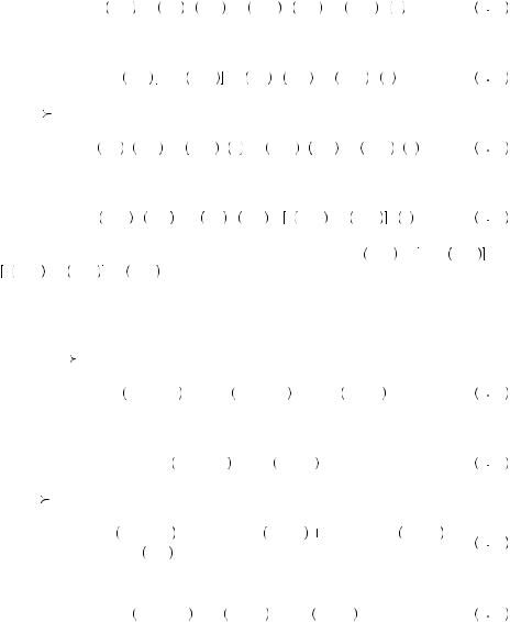
Jacob Marschak and Mark Machina). The x-axis in the figure represents the probability of wining $0, and the y-axis represents the probability of winning $100. The probability of a third outcome, winning $50, is not pictured on an axis. Thus, each point in the triangle represents a lottery with the probability of winning $0 represented by the x- coordinate, the probability of winning $100 represented by the y-coordinate, and the probability of winning $50 equal to the remaining probability (one minus the x- and y- coordinates). The points along the x-axis represent gambles in which the probability of winning $100 is 0. Thus all points on this line represent gambles that could result in winning either $50 or $0. The point (0,0) represents the gamble yielding $50 with certainty. The point (1,0) represents winning $0 with certainty. The points along the y- axis represent all gambles with a probability of 0 of winning $0. The point (0,1) represents the gamble that yields $100 with certainty. The dashed line running from the upper left to the lower right portion of the graph represents the boundary of the triangle. Along this boundary the sum of probabilities of $100 and $0 outcomes is 1, and thus the probability of winning $50 is 0.

The parallel lines stretching from the lower left to the upper right represent indifference curves in the triangle. The indifference curve containing all points yielding utility identical to receiving $50 with certainty is labeled. Because we have placed the probability of $100 on the y-axis and $0 on the x-axis, all indifference curves to the left of this curve represent a higher level of utility than $50 and all to the right represent a lower level of utility. You will note that all indifference curves are parallel and straight lines. Let y be the probability of winning $100 and x be the probability of winning $0. In the triangle, an indifference curve is all probabilities y and x that satisfy

Solving equation 9.14 for y in terms of x yields

Because the value k and the utilities are fixed, this always represents a line with slope given by

Thus, expected utility theory implies that all indifference curves must be straight lines, with each having the identical slope. This property drives many of the tests of expected utility theory.

Note that the slope of the line in equation 9.15 is made up of the ratio of the difference in utility between $50 and $0 to the difference in utility between $100 and $50. Recall from Chapter 6, that a person’s risk preferences are related to the curvature of the utility of wealth function. The greater the gambler’s level of risk aversion, the more the slope of his utility function declines as wealth increases. If the gambler is risk averse, we should

observe that the rise of the utility function from $0 to $50 is larger than the rise from $50 to $100 (both intervals have a run of $50 needed to complete the standard formula for slope). More generally we can measure this decline in slope through the ratio of u50 − u0 to u100 − u50. Greater risk aversion means that u100 − u50 is smaller relative to u50 − u0, implying a larger value in the right side of equation 9.16. Thus, the more risk averse the preferences, the greater the slope of the indifference curves. This is always the case when the x and y axes contain the highest and lowest value outcomes, respectively.

EXAMPLE 9.4 Allais’ Paradox

Maurice Allais was one of the earliest to criticize the expected utility model of decision under risk, believing it eliminated many of the important psychological factors involved in risky decisions. He made the argument using hypothetical choices between gambles that most readers would acknowledge seem to call expected utility theory into question. For example, suppose you had to choose between:

Now suppose you were deciding between

Many choose A rather than B because of the certainty of receiving something from the gamble. However, very few would choose C over D because the 1 percent additional probability of winning something in C does not feel as if it compensates for the reduction in payoff from $500 to $100.

But these two decisions contradict the rational axioms. Note, A B implies that

which clearly contradicts equation 9.17. This is often called the Allais’ paradox or the common outcome effect.

The term common outcome effect refers to the structure of the gambles. Gambles A and C can be thought of as probability 0.11 of receiving $100 and probability 0.89 of receiving $X, where in A, X = 100 and in B, X = 0. Gambles B and D can be thought of as probability 0.1 of receiving $500, probability 0.89 of receiving $X, and probability 0.01 of receiving $0, where in B, X = 100, and in D X = 0. In all gambles, X is the common outcome (has the same value and probability in both choices). Expected utility theory implies that the value of X should not affect the gambler’s choice. However, here we have observed that people change their preference depending on whether X is 100 or 0. Economics experiments have repeatedly found evidence of the common outcome effect in risky choice.

This is a violation of the independence axiom. This is relatively easy to see in the Marschak–Machina triangle, as seen in Figure 9.3. Gambles C and D are created by sliding gambles A and B to the right by 0.89 (increasing the probability of $0 by 0.89). The line segment AB is exactly as long and of the same slope as line segment CD. Recall that under the independence axiom, indifference curves in the Marschak–Machina triangle are straight parallel lines sloping upward. Further, preferred gambles should lie to the northwest of the indifference curves. If D is preferred to C, then indifference curves must be of a slope that could place D to the northwest and C to the southeast (as pictured). However, it is impossible to find a line of identical slope that would place A to the northwest and C to the southeast. Thus, the indifference curves must change slope in different parts of the triangle, with steeper indifference curves to the west. This is a common method for finding risky choices that violate the independence axiom.

Allais’ choice problem is also an example of the certainty effect. The certainty effect is the name applied to choices in which decision makers display an irrational preference for outcomes with certainty. For example, in this case it might be that A is chosen

p(500) = 1

Probability of $500

B D

because of the certainty effect, even though gambles that have the same relationship in the Marschak–Machina triangle that do not involve certainty (such as C and D) would display the opposite preferences. This observation that people tend to violate the independence axiom often in preference of a certain outcome has led to the hypothesis that people do not perceive probabilities as summing to 1. Rather, they perceive a probability p of outcome X as yielding πp probability of receiving utility UX, where πp is such that πp + π1 − p < 1, called subadditivity. Thus, uncertain outcomes are discounted relative to certain outcomes. In this framework, called probability weighting, A B implies

weighting is a way to represent systematic misperception of probabilities in choice preferences. Thus, subadditivity may be one explanation for the common outcome effect.

Chris Starmer is among a group of economists who suggest regret aversion may be behind the common outcome effect. Using the case above, if the gambles were inde-

Equations 9.27 and 9.26 are not contradictory so long as U0, 500 is sufficiently negative. In this case the person would feel so much regret from obtaining zero if 500 would have been drawn otherwise that their preferences reverse. Starmer and others have found some evidence that the common consequence effect and related behavior is due to the possibility of regret.

EXAMPLE 9.5 Common Ratio Effect

Allais also discovered the common ratio effect. Consider the following choices (from

Kahneman and Tversky).

Now suppose you were deciding between

Kahneman and Tversky found that about 80 percent of those asked would choose Gamble A, and about 65 percent would choose Gamble D. However, choosing A and D is a violation of expected utility. To see this, note that A B implies

Clearly, equations 9.30 and 9.28 cannot both hold. This is the common ratio effect again because of the structure of the gambles involved. Gamble C can be thought of as a 0.25 chance of playing gamble A and a 0.75 chance of receiving $0. Similarly, Gamble D can be thought of as a 0.25 chance of receiving gamble B (resulting in 0.20 probability of $4,000) and a 0.75 chance of receiving $0. Thus, the ratios of the probabilities of outcomes in gambles A and B remain the same in gambles C and D, with a common outcome added. This particular version of the common ratio effect may also be thought of as an example of the certainty effect given the involvement of Gamble A.