Conjunction Bias

As participants rank these possibilities in their mind, they are drawn to the description of Linda and tend to rank the items in order of how representative of each item that description is. Thus, participants might have felt that relatively few bank tellers are deeply concerned with social justice, and thus this outcome is thought to be improbable. But if we think about feminist bank tellers, this group is probably much more concerned about social justice, and thus people consider this event to be more likely. This is called the conjunction effect. By intersecting relatively unrepresentative events (bank teller) with very representative events (feminist), the conjunction of the two is considered more probable than the unrepresentative event because the description is more representative of the combined events. Such effects may be related to the heuristics and biases that lead to stereotyping, bigotry, or other potentially undesirable phenomena. This possibility is discussed later in the chapter.

EXAMPLE 7.4 Calling the Election Early

The 2000 presidential election was notable for how difficult it was to determine the winner. In fact, it took more than a month and several legal actions before the Supreme Court finally declared George W. Bush to be the winner of the election. The confusion all centered around the vote count in Florida. Should Florida be called for Bush, Bush would have the necessary electoral votes to become president. If instead Florida were called for Albert Gore, Gore would have enough electoral votes to become president.

Election night was particularly interesting. In most modern elections, news media cooperated under the banner of Voter News Service (VNS) to compile exit polls to determine a winner. Voters were interviewed as they left the polls and asked how they voted. These numbers were then reported to the news media, and usually the news networks would project a winner of the election when they had determined they had enough data to make a prediction. News programs are very careful not to call a state for one particular candidate until they are certain they know the outcome. Their reputation as a reliable news source depends on this accuracy. From years of experience, television viewers had come to expect a declaration of a winner before they went to bed on election night. Come election night 2000, almost every state fell to the expected can- didate—the candidate who had polled better in each state—but something strange happened in Florida.

Early in the counting, 7:50 P.M., the news networks predicted Gore was a lock to win Florida. Later, at 9:54 P.M., the networks retracted that lock and called the outcome ambiguous. Later, at 2:17 A.M. the next day, they stated that Bush was a lock to win Florida and the election. At this point Gore decided to concede the election to his rival. He called George W. Bush and congratulated him on the outcome. A short time later, Gore called to retract his concession in what must have been a truly awkward exchange. At 3:58 A.M., the networks retracted their projection of Florida and said the outcome of the election was ambiguous. Similar reversals happened in a couple other states as well, but neither of these was important to the outcome of the election. In response to this debacle, VNS was terminated, and news agencies began holding their projections until

vote totals were certified by election officials. What led to these historic and misleading reversals? How could the prognosticators from the major networks get their statistics so incredibly wrong?

The final official vote count was 2,912,790 to 2,912,253 in favor of Bush, with 138,067 votes for other candidates. Vote totals for the moment when the election was called for Gore are not available. However, when the election was called for Bush, he had a 50,000 vote lead. So, at what point do you gain confidence enough in a trend to make a prediction? The true distribution of legal votes (ignoring votes that could not be verified) was 48.85 percent for Bush, 48.84 percent for Gore, and 2.31 percent for other candidates. When making such a forecast, we should make our prediction when we can say that the vote total we currently observe is improbable if the true vote total were to be a tie.

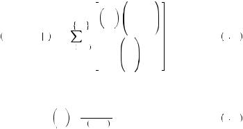
Let’s suppose we had 6,000,000 colored balls in a jar. For simplicity let’s suppose some are red and some are white (so no other candidates). We start pulling these balls out of a jar, and at some point, when we have drawn n > 50,000, we observe 50,000 more red than white. What is the probability of a tie given our observation? The formula for calculating such a thing is actually quite complicated. Let nr be the number of red balls drawn, nw the number of white balls drawn, n be the total number of balls drawn, and N be the total number of balls in the jar. Suppose that there are equal numbers of red and white balls in the jar (a tie). We can write the probability that there are k more red balls that have been drawn than white balls as

is the number of orderings in which x objects can be drawn from a total of y objects. This formula is somewhat difficult to calculate with large numbers. To simulate, let us suppose there are only 600 voters, with 300 voting for Bush and 300 voting for Gore. Here, a difference of 50,000 is equivalent to a difference of just five votes. Table 7.1 displays the probability of observing a five-vote difference in favor of red for various total numbers of balls drawn.

From Table 7.1, the probability of observing a five-vote difference does not drop below 20 percent until one has drawn and counted at least 550 of the 600 balls in the jar. If we scale these numbers back up to our original voting problem, it appears that probability of observing a difference of 50,000 would not drop significantly until you have counted the equivalent of 5,500,000 of the ballots. This is a poor approximation of the probabilities for 6 million ballots, but it will do for our purposes. The news networks

Table 7.1 The Probability of a Five-Vote Difference for Various Sample Sizes

were making projections based on precinct-by-precinct data. They only received the data as the precinct polls closed and local votes were tallied. The problem they ran into was taking account of the order of the reports.

They first received reports from suburban precincts in the east that voted mostly for Gore. Thus, if they anticipated early data to arrive from Gore precincts, they should have expected an early large lead for Gore. When the rural (Bush) districts in the west began reporting, suddenly Bush erased Gore’s lead and built a 50,000-vote lead. But results still had not been reported from the urban (Gore) centers in Miami and other cities where voting totals take longer to count. The networks used a projection trigger that must have well overstated the probability that the observed trends would hold. At the time the vote was called for Bush they should have known that a 50,000 vote lead with large and heavy Gore territory still to come was not good enough for prediction. In fact, there was less than a 70 percent chance that the lead would hold. Simply put, this decision was made way too early, but despite knowing and using statistical models, they made this call.

The Law of Small Numbers

In general, psychologists and economists have found that people tend to believe that small samples from a distribution will be very similar in all respects to the population from which they are drawn. The law of large numbers tells us that when we have large numbers of observations, the sample mean of our observations will converge to the true mean. In this way, when we have a large sample of observations, it is very likely that the properties of this sample will resemble the population from which it is drawn. However, small samples do not provide the same guarantee. If we were to toss a fair coin four times, it is more likely that we should observe an outcome with either zero, one, three, or four heads than one with exactly two heads. Nonetheless, people believe that the outcome with two heads, which is most representative of a fair coin toss, is more likely than it truly is.

This tendency to exaggerate the probability that a small sample is representative of the underlying process that generated it has been facetiously named the law of small numbers by Amos Tversky and Daniel Kahneman. As the name suggests, people treat small samples of data as if they were dealing with much larger samples of data. Thus, for example, one might rely too heavily on trends in early voting when predicting the outcome of an election. Similarly, one might rely too heavily on performance data over a short period of time. For example, each year a list of mutual funds that had the highest return in the last year is widely circulated in the financial press. Many people select which mutual funds to purchase based upon this list. However, it is very seldom that the results for any year are good predictors of performance in the future. For example, only three of the top 10 mutual fund families for 2008 were also in the top 10 for 2007. Even when we consider the top performer over five years, only four of the top 10 remained on the list in both 2007 and 2008. Such a high level of volatility suggests that performance may be almost entirely random. Nonetheless, people behave as if the differences are systematic because the small sample is taken to be representative of the true underlying differences in mutual fund performance.

Matthew Rabin has proposed a behavioral model of learning according to the law of small numbers. It will be helpful to first describe his model intuitively. Suppose we are considering the repeated flipping of a fair coin. We know the probability of a heads is 0.5 for any flip, and we know that this probability does not depend on whether heads or tails was drawn previously. We can represent the beliefs of someone regarding what will be drawn as a distribution of balls in an urn containing N balls. I will refer to this as the mental urn to emphasize that it is merely a concept used in modeling and does not truly exist. Half of the balls are labeled “heads,” representing the probability that a heads would be tossed, and half of the balls are labeled “tails.” This person believes that a sequence of tosses should be representative of the true underlying probability and thus should display about half heads. Each toss draws one of the balls from the urn.

Suppose the mental urn originally contained six balls, with three labeled “heads” and three labeled “tails.” The original beliefs are thus that the probability of a heads is 3/6 = 0.5. Suppose then that the first coin is tossed and it comes up heads. This removes one of the balls labeled heads from the mental urn, so that the beliefs for the next toss are that the probability of a heads is 2/6 0.3. Thus, when a heads is tossed, this observer feels that it is more likely that a tails will be tossed to balance out the sequence, making it more representative of the overall probability.

Further, Rabin supposes that the mental urn is refreshed periodically, for example after every two tosses. In this process, the number of balls in the mental urn determines how biased the observer may be. For example, if we had considered a mental urn with 1,000 balls, the bias would be very small. In this case, after tossing one heads the believed probability of a heads moves from 0.5 to 0.499. On the other hand, if the number of balls in the mental urn were two, the believed probability would move from 0.5 to 0. This process results in a belief that draws are negatively correlated when in actuality they are independent. Thus, the observer believes heads are more likely following tails than following heads. In actuality the probability is always 0.5 regardless of whether a heads or tails has recently been tossed. Refreshing the balls in the mental urn has the effect that the law of small numbers is applied locally to a series of draws rather than to the overall process. This can be considered the sample window for the law of small numbers.

720

In this case, Freddie feels it is too improbable that a good fund would have two bad years in a row. Once the second bad year in a row is realized, Freddie immediately believes there is no chance that he could be observing a good fund. He thus would choose not to invest, when in fact there is a higher probability that he is dealing with a good fund than a bad fund. Adjusting the size of the mental urns so that they are larger brings the result more closely in line with Bayes’ rule. Further, refreshing the urns less often (while holding the number of balls constant) leads to a greater expectation of correlated draws before refreshing the urn. Thus, Freddie will infer more and more information from the second, third, or fourth draw before the mental urns are refreshed. Note in this example that the “good fund” was excluded on a second draw for exactly this reason.

In general, the law of small numbers leads people to jump to conclusions from very little information. Early counts from a sample will be taken as overly representative of the whole, leading to snap judgments. When making judgments based on data, it is important to consider the true variability and the amount of information contained in any sample of data. Early judgments may be based on an odd or nonrepresentative sample. Further, one must be aware that others are likely to judge their efforts based on small and potentially unrepresentative samples of their output. Thus, a newly hired worker might do well to put in extra hours early on when initial judgments are being formed.

EXAMPLE 7.5 Standards of Replication

In scientific inquiry, replication forms the standard by which a research discovery is validated. Thus, one scientist tests a hypothesis using an experiment and publishes the results. Others who may be interested validate these results by running identical experiments and trying to replicate the outcome. But what constitutes replication?

Earlier in this chapter we reviewed the mechanics of a statistical test. Nearly all experimental results are reported in terms of a statistical test. For example, a scientist may be interested in the effect of a treatment (say, the presence of chemical A) on a particular population (say, bacteria B). Thus, he would take several samples of bacteria B and apply chemical A under controlled conditions. He would also take additional samples of bacteria B and keep them in identical controlled conditions without introducing chemical A. He would then measure the object of his hypothesis in each sample. For example, he may be interested in measuring the number of living bacteria cells remaining after the experiment. He would measure this number from each sample and then use statistics to test the initial hypothesis that the means were equal across the treatment and control samples.

Typically, scientists reject this hypothesis if there is less than a 5 percent chance of observed difference in means, given the true means were equal. This is generally tested using a test statistic of the following form

In truth, if we conducted a new study and found t = 1.70, this should strengthen our confidence in the results of the previous study, now being able to reject the initial hypothesis at the α = 0.0056 level. Instead, the psychologists believed the second study contradicts the first. Owing to belief in the law of small numbers, they believe that if the first study were true, the second study should have an extremely high probability of producing a test statistic that is very close to the statistic in the first study. In fact, they exaggerate this probability. In other words, they believe the data should be more representative of the underlying process than it truly is given the small sample sizes.

Similar questions asked the psychologists to consider a student who had run an experiment with 40 animals in each of two treatments, finding a test statistic of 2.70. The result was very important theoretically. The psychologists were asked to consider whether a replication was needed before publication, and if so, how many observations would be needed. Most of the psychologists recommended a replication, with the median number of recommended subjects being 20. When asked what to do if the resulting replication produced a test statistic of only 1.24 (which cannot reject the initial hypothesis of equal means) a third of the psychologists suggested trying to find an explanation for the difference between the initial study subjects and the subjects included in the replication. Tversky and Kahneman note that the statistical difference between the initial group and the replication group was incredibly small. The treatment effects in the replication are about 2/3 of the treatment effects in the initial sample. Trying to explain this difference is like trying to explain why a penny came up heads on one toss and tails on another. The differences are almost certainly due to random error. Nonetheless, believers in the law of small numbers can attribute even small differences in very small samples to systematic causes. In the pursuit of scientific progress and publications, this can have disastrous consequences. There are numerous examples of early medical studies where failure to understand the statistics of replication has done real harm to people.

EXAMPLE 7.6 Punishments and Rewards

The representativeness heuristic can lead people to believe in causal effects that are nonexistent. For example, suppose you managed a flight school. Psychologists have generally suggested that positive reinforcement, or rewarding good behavior, is an effective tool in teaching. Hence, you decide to reward trainees after a particularly good flight. After several months of this policy, you begin to notice that after each pilot has

been rewarded for a good flight, their next flight tends to be worse—sometimes much worse. In fact, almost no rewarded pilot has ever improved in the next following flight. Seeing this, you begin to question the psychologists and revamp your policy. Now, instead of rewarding good flights, you decide to punish bad flights. Again several months pass and you begin to evaluate the results. This time you are satisfied to learn that students almost always improve after receiving punishment. Clearly this must be a very effective policy.

In fact, Daniel Kahneman and Amos Tversky put a similar question to a sample of graduate students and found that all agreed with the logic of this story. This example arose out of Daniel Kahneman’s experience in the military in which flight instructors had concluded that reward leads to worse performance and punishment leads to better performance. Yet, in flight training one is very unlikely to make much improvement from one flight to the next. Progress takes a long time. Thus, big changes in performance are most likely due to random variation in conditions (e.g., weather, task, individual rest or alertness) rather than changes in skill. Thus, a particularly good flight is almost certainly due to a very lucky draw. Suppose the probability of an especially good flight was 0.10. If rewards and punishment had no effect on pilots’ performance, following any good flight there would be a 0.90 chance of doing worse on the next flight. As well, if there was a 0.10 chance of a particularly bad flight, then there would be a 0.90 chance of improving on the next flight. This is called reversion to mean. Performance near the mean or average is the most probable outcome. Thus, high performance is most likely to be followed by low performance, and low performance is most likely to be followed by high performance. However, people have a hard time perceiving reversion to the mean as a possible cause in this case.

In a more general context, reversion to the mean can appear to be some mysterious but systematic cause of apparently random events. For example, suppose you observed a slot machine over time. Because of reversion to the mean, you would notice that after a large payout, the machine is likely to return a smaller payout on the next pull. Further, if you observed a zero payout (which is most common), there is a higher probability of a higher payout on the next pull. This could lead you to reason that you should play slot machines that haven’t given a prize recently, and switch machines if you win anything. This, of course, is statistical fallacy. In truth, the probability of each possible payout is the same on each pull. It is not the probability of an $x payout that has increased or decreased; this remains the same with each pull; rather, it is the probability of a higher or lower payout than the previous pull. Because the previous pull is a random event, it is the threshold that determines what is higher or lower that is moving. If you feel that playing a slot machine after a zero payout pull is a reasonable gamble, you should also be willing to pull after a large payout on the same machine.

Rabin’s model of beliefs can be used to model this anomaly. Suppose the gambler has a mental urn with 10 balls, one labeled “win” and nine labeled “lose.” With each play, a ball is drawn from the mental urn, adjusting the perceived probability of a win on the next pull. After a series of zero-dollar payouts (lose), the probability of a win increases. After a single win, the gambler might perceive that there is a zero probability of a second win, and thus stop. Thus, the law of small numbers can lead people to misinterpret a series of random numbers, leading them to believe they are systematic.

EXAMPLE 7.7 The Hot Hand

In watching a basketball game, it is hard not to be amazed by the long streaks of shots made by the best players. Often sportscasters keep track of how many shots a particular player has made in a row without missing. In fact, 91 percent of basketball fans believe that after a player has made one shot, he has a higher probability of making the next shot. This leads 84 percent of basketball fans believe that it is important to get the ball into the hands of a player who has made several shots in a row.

Thomas Gilovich, Robert Vallone, and Amos Tversky used videotapes of basketball games as well as records to test for shooting streaks. Their analysis focused primarily on the Philadelphia 76ers; however, similar results were found with the New Jersey Nets and the New York Knicks. In interviewing the 76ers themselves, they found that the players believed in systematic shooting streaks. Players said that once they have made a few shots in a row, they felt they could not miss. Gilovich, Vallone, and Tversky then used data collected over an entire season to calculate the percentage of shots hit given the previous performance. If the player had just missed one shot, he hit 54 percent of his next shots. If the player had just hit one shot, he hit 51 percent of his next shots. After hitting two shots, his probability was 50 percent. Basketball fans, when surveyed, had expected a 50 percent shooter to have a 61 percent chance of making a second shot once the first was made. The estimated correlation coefficient between the outcome of one shot and the next was −0.039. This value is small enough that it is not statistically different from zero, suggesting that streaks are an illusion. Each shot is essentially independent of the previous shot. They are unrelated draws from the same distribution. Gilovich, Vallone, and Tversky also analyzed game-by-game shooting percentages to see if a player’s performance in a single game could be distinguished from any other game. Similarly, they found no evidence that players have hot and cold shooting nights. They also found no evidence that free-throw shooting follows streaks. For example, Larry Bird, in the 1980–81 season, made 91 percent of his free throws that followed a missed free throw, and he only made 88 percent when following a hit free throw.

The Cornell University basketball team was enlisted to test the hot hand theory that players go on hot or cold streaks. Players were paired up. One would shoot and the other would observe the shooter. Each was allowed to bet either a high or low amount on each shot. If they bet the low amount they would win 2 cents for a made shot and lose 1 cent for a missed shot. If they bet high, they would win 5 cents for a made shot and lose 4 cents for a missed shot. The bets of both the shooters and the observers were highly correlated with the outcome of the previous shot. Thus, they bet high more often when the previous shot was made. However, predictions were relatively unrelated to the outcome of the shot being predicted. Several analyses have found that the perception of the hot hand affects the betting markets for teams that are on winning streaks. The point spread necessary for a win widens as the team lengthens it streak. Yet the wider the point spread, the higher the probability that the team loses.

Clearly, both players and fans misperceive the relationship between shots taken. In fact, after publication of this study there was a fair amount of outrage on the part of coaches. Several prominent coaches from both the pro and college ranks criticized the findings heavily. For example, Bobby Knight was prominently quoted in the newspapers suggesting that the researchers did not understand the game. Alternatively, we might

consider these coaches to be operating with a mental urn that is too small. People infer too much information from the streak of hits that are entirely consistent with shooting averages. Rather, they believe they are drawing from a more favorable mental urn—an urn representing an event that does not actually exist.

EXAMPLE 7.8 The Gambler’s Fallacy

When playing the roulette wheel at a casino, a wheel with red and black sections is spun, and gamblers place bets on the color of the section that will come to rest under a pointer. Clearly, each spin is an independent random event, and state gambling commissions verify the fairness of the equipment on a regular basis.

Rachel Croson and James Sundali observed casino gamblers placing bets on a roulette wheel. They found that, for example, if red had been spun on the previous spin, or even up to the previous three spins, people tended to bet about 50 percent of the time on red and about 50 percent of the time on black. However, when the number of spins has reached four in a row, people start betting against the streak. After four in a row of black, about 58 percent bet red. After five in a row of black, about 65 percent bet red. After six or more in a row of black, 85 percent bet red. Nonetheless, a black or red draw is just as likely after six black spins in a row as it is after one black spin in a row. This phenomenon is called the gambler’s fallacy. In this case, people know the probability of each outcome, and they believe (according the law of small numbers) that the draws should even out to the correct proportions over time. Thus, they begin to bet more and more heavily on the outcome that has appeared least.

At first glance, this might appear to be the exact opposite of the hot hand bias. In the hot hand, a streak leads one to bet on continuing the streak. In the gambler’s fallacy, a streak leads one to bet against the streak. The key difference is that in the hot hand bias, there is not a known probability. Thus, the gambler is trying to infer the probability from the performance. Hence, according to Rabin’s model, the gambler is trying to figure out which mental urn best represents the data. The particular mental urn chosen might change as the result of a streak if the mental urns are small. Alternatively, under the gambler’s fallacy the probability of each outcome is transparent. For example, a standard roulette wheel has 18 red sections, 18 black sections, and two green sections. Each section is of identical size, resulting in a probability of red of about 47 percent. In this case, the gambler knows what mental urn he is drawing from but uses the remaining contents of the urn to predict the future outcomes. Thus, the more red draws, the fewer red balls in the mental urn and the higher the probability of a black on the next draw. The same pattern can be observed in the play of state lotteries. After a winning number is drawn, the number of people choosing that number in the next day’s lottery falls by roughly one third, and it remains below normal for close to a month (or until the number is drawn again).

Another interesting and potentially related anomaly has been found in lottery play. People ascribe more value to a ticket when they are allowed to choose the numbers than when the numbers are chosen for them. Ellen Langer conducted a study in which she sold lottery tickets to about 50 people under the guise of a Super Bowl–themed lottery. Each lottery ticket had the picture of a professional football player on it and a