

|
|
|
|
|
348 |
|
COMMITTING AND UNCOMMITTING |
Odysseus further commands his men to tie him to the mast so that he cannot escape. While thus tied to the mast, he could be exposed to the temptation but would not have the choice to steer the ship toward the Sirens’ song. He could thus become the only man to have heard their song and lived. By restricting his choice set, he could indulge in the song without giving in to the temptation that accompanied it. In this case, he could consider himself better off for making the commitment because he expected to do something that would harm him if he was not thus committed. In other words, Odysseus must have believed he would make the wrong choice in order for being tied to the mast to make sense. In a similar sense, commitment mechanisms can be used by those who recognize their own time inconsistency to tie themselves to the mast.
Rationality and the Possibility of Committing
The fully additive exponential model of discounting predicts that people will display time-consistent preferences. In this case, people would have no desire to precommit to a specific path because they know they would eventually take that preferred path anyway. There is no temptation to do anything else in the rational model. Consider again the fully additive model presented in Chapter 12, in which the decision maker solves
max U c1, c2, |
= max |
T |
δi − 1u ci |
13 1 |
|
i = 1 |
|||||
c1,c2, |
c1, c2, |
|
|
||
|
|
|
subject to whatever budget constraint he faces. This model assumes that consumers determine their entire consumption path, the consumption quantity for each individual time period, all at the initial time period. Thus, this model in reality assumes that the consumer can commit to the consumption path that solves equation 13.1. If instead we are attempting to model the case in which consumers cannot commit to a consumption path, then the model must reflect that consumers decide on the level of consumption in this period based upon what they believe they will decide to do in the future. Thus, in period t, the consumer solves the recursive optimization problem:
maxct <wt u ct + δ maxct + 1<wt + 1 u ct + 1 + δ2 maxct + 2<wt + 2 u ct + 2 + |
, 13 2 |
where wt is the budget constraint in period t that depends on consumption in all prior periods.
Equation 13.2 can be a little difficult to interpret at first. Consumers maximize their utility of consumption in this period given that they will behave so as to maximize their utility of consumption again in each future period as well. This may be easiest to see in a finite horizon problem. Consider consumers who have initial wealth w and must allocate it to consumption over three periods. After the third period, they will die, and no further consumption will be possible. Further suppose that the cost of one unit of consumption is one unit of wealth. Then, when consumers are deciding on consumption in the first period, they anticipate the maximization problem they will face in the second and third periods.

|
|
|
|
Rationality and the Possibility of Committing |
|
349 |
|
A fully continuous problem for the general consumption case is presented in the Advanced Concept box at the end of the chapter. For a simple example, consider the discrete-choice problem where, in the first and the second period, laborers can either decide to work, receiving instantaneous utility of w, or shirk, receiving instantaneous utility of s, where s > w. In the third period, the laborers receive $10 for each day they worked, yielding instantaneous utility u 10x
10x = 10x, where x is the number of days worked. In the third period, the laborers have no actions they can take, and thus they simply receive instantaneous utility of the payment. If we consider the choice the laborers face in the second period, given their action in the first period, they must solve
maxz2 = w,s z2 + δ × 10x, |
13 3 |
where zi is the action chosen in period i, and
2 |
if |
z1 = w, z2 = w |
|
x = 1 |
if |
z1 = w, z2 = s . |
13 4 |
1 |
if |
z1 = s, z2 = w |
|
0 |
if |
z1 = s, z2 = s |
|
They will choose to work so long as
w + δ x1 + 10 > s + δx1, |
13 5 |
where x1 is the reward resulting from the action chosen in the first period. This can be rewritten as
10δ > s − w. |
13 6 |
Let us suppose that this is the case, so that no matter what was chosen in the first period, laborers will choose to work in the second period. Then, in the first period, laborers face the problem
maxz1 = w,s
w,s z1 + δ maxz2 =
 w,s
w,s
 z2 + δ × 10x
 = maxz1 =
 w,s
w,s z1 + δw + δ2
 x1 + 10
 ,
,  13
13 7
7
where the second and third terms result from the laborer choosing to work in the second period regardless of the first-period decision. The laborer will decide to work in the first period if
w + δw + δ220 > s + δw + δ210 |
13 8 |
or, rewriting, |
|
10δ2 > s − w. |
13 9 |
|
|
|
|
|
350 |
|
COMMITTING AND UNCOMMITTING |
Let us suppose that this is not the case, but that the laborer decides to shirk because 10δ2, the discounted reward for working in the first period, is less than the immediate difference in utility between working and shirking, s − w. For example, suppose s = 3, w = − 2, δ = 0.7. Then, from equation 13.6, 10δ = 7, which is greater than s − w = 5, implying the laborer will decide to work in the second period. However, 10δ2 = 4.9, which is less than s − w = 5. Thus, according to equation 13.9, the laborer would choose to shirk in the first period. Thus, the recursive optimization problem results in the laborer choosing to shirk in the first period, working in the second period and receiving $10 in pay in the third period.
This method of solving for the optimal sequence of decisions is called backward induction, and it is commonly used by economists to model decision makers’ anticipation of behavior (either their own or others’) in future periods. This model essentially assumes that the laborer will optimize in each period, conditional on assuming he will reoptimize in each subsequent period. Backward induction is most often used by economists to model games involving sequential decisions by multiple players. In the case of a potentially time-inconsistent decision maker, it may be thought of as a game involving decisions by several different selves, one for each period of the optimization. Backward induction yields the optimal plan, taking account of the potential for timeinconsistent preferences. In the case of exponential discounting, however, the decision maker should not display time-inconsistent preferences.
To see this last point, consider the standard fully additive model from equation 13.1. In the framework of our laborer, in the first period he would simply solve
maxz1,z2 w,s z1 + δz2 + δ210x. |
13 10 |
In this problem there are several possibilities, and the utility of all possible choices can be written as
|
w + δw + δ220 |
if z1 = w, z2 = w |
|
|
U z1, z2 = |
w + δs + δ210 |
if |
z1 = w, z2 = s |
|
s + δw + δ210 |
if |
z1 = s, z2 = w . |
13 11 |
|
|
s + δs |
if |
z1 = s, z2 = s |
|
Note from equation 13.11 that the possible choices  z1 = w, z2 = w
 and
and  z1 = s, z2 = w
 are identical to the choices from the recursive problem in equation 13.7. Among these two options, the laborer would again choose
  z1 = s, z2 = w
 , indicating no time-inconsistent preferences. If there is any chance for time-inconsistent preferences, it must come from one of the other options. But each of the other options is clearly dominated by one of the two choices from equation 13.7. Choosing
  z1 = s, z2 = s
 could only happen if
s + δs > s + δw + δ210, |
13 12 |
the utility resulting from  z1 = s, z2 = w
 , which implies that 10δ < s − w. But this contradicts our assumption from equation 13.6. Choosing
  z1 = w, z2 = w
 could only occur if

 . In fact these are identical, and thus decision makers should not be willing to give up anything to obtain a commitment mechanism.
|
|
|
|
|
352 |
|
COMMITTING AND UNCOMMITTING |
People without access to a credible way to commit to future acts must then anticipate their future actions by solving the recursive optimization problem. Only now, because of the quasi-hyperbolic discount function, the problem becomes somewhat more complicated than that written in equation 13.2. Instead, the decision maker must solve
maxc1 u c1 + |
T |
βδi − 2u ci* , |
13 15 |
i = 2 |
where c*i is defined recursively as solving
maxc |
u ci + |
T |
βδ j − 2u |
c* |
, |
13 16 |
|
j = i + 1 |
|||||||
i |
|
|
j |
|
|
where the budget set in each period is conditioned on the consumption decisions from previous periods. We refer to decision makers who behave as if they solve the recursive optimization problem as sophisticated, and we refer to those who solve the standard maximization problem (as in equation 13.1) as naïve or committed, depending on the context. Sophisticated decision makers anticipate their future behavior, and naïve decision makers do not consider how their future plans will change based upon changes in how they discount a particular period relative to other periods. Alternatively, those who can commit to a particular consumption path will also solve equation 13.1 because they need not worry about their future behavior. The commitment mechanism ensures that behavior conforms to their current preferences.
To develop some intuition about what this model means, consider the three-period model from the previous section, only now suppose that the laborer discounts according to the quasi-hyperbolic model, with parameters β and δ. We can solve this problem by backward induction as before. In the third period, laborers face no choices but just receive the reward for their prior actions. Thus we begin by considering the choice from the point of view of second-period laborers. In this case, laborers will solve
maxz2 = w,s z2 + β × 10x. |
13 17 |
They will choose to shirk so long as
w + β x1 + 10 < s + βx1, |
13 18 |
where x1 is the reward resulting from the action chosen in the first period. This can be rewritten as
10β < s − w. |
13 19 |
Let us suppose that this is the case. Then the laborer chooses to shirk in the second period no matter what happens in the first period. Then, in the first period, the laborer would solve
maxz1 = w,s
w,s z1 + β maxz2 =
 w,s
w,s z2 + δ × 10x
 = maxz1 =
 w,s
w,s z1 + βs + βδx1,
  13
13 20
20

|
|
|
|
Commitment under Time Inconsistency |
|
353 |
|
where the second and third terms result from the laborer choosing to shirk in the second period regardless of the first-period decision. The laborer will decide to work in the first period if
w + βs + βδ10 > s + βs |
13 21 |
or, rewriting, |
|
10βδ > s − w. |
13 22 |
But if equation 13.19 holds, clearly equation 13.22 cannot. Thus, the laborer would choose to shirk in both periods and earn no reward.
We can contrast this solution with the choice made if the laborer could commit to his work plan in the second period without the possibility of changing his mind. Then, the laborer in the first period would solve
maxz1,z2 w,s z1 + βz2 + βδ10x. |
13 23 |
Proceeding as in the previous section, this is equivalent to maximizing the function
|
w + βw + βδ20 |
if z1 = w, z2 = w |
|
|
U z1, z2 = |
w + βs + βδ10 |
if |
z1 = w, z2 = s |
|
s + βw + βδ10 |
if |
z1 = s, z2 = w . |
13 24 |
|
|
s + βs |
if |
z1 = s, z2 = s |
|
In this case, the choices  z1 = w, z2 = s
 and
and  z1 = s, z2 = s
 are identical to the choices that were available to the first-period decision maker using backward induction in
equation 13.20, and thus clearly  z1 = s, z2 = s
 would dominate between these two
options. But the other two options were not available. The option |
z1 = w, z2 = w would |
||
be chosen if w + βw + βδ20 > s + βs, or, rewriting, |
|
||
|
βδ |
|
|
20 × |
|
> s − w. |
13 25 |
1 + β |
|||
Given that equation 13.22 holds, this could only be the case if 2 1 + β
1 + β is much greater than 1.
Let us suppose that this is not the case. For example, suppose s = 3, w = − 2, δ = 0.7, β = 0.5. Then,
20 × |
βδ |
4.67 < s − w = 5, |
13 26 |
1 + β |
implying that the laborer would prefer to shirk in both periods than to work in both periods. The remaining choice,  z1 = s, z2 = w
 , would be chosen over the other options

|
|
|
|
|
|
354 |
|
COMMITTING AND UNCOMMITTING |
|
|
|
if s + βw + βδ10 > s + βs, or, rewriting, if δ10 > s − w. Using the numerical example, this |
||
|
|
would hold because δ10 = 7 > s − w = 5. Thus, given the option to bind himself to a work |
||
|
|
plan in the future, the laborer will choose to shirk today and work tomorrow. Of course, |
||
|
|
he will not really want to work when tomorrow comes, but his commitment eliminates |
||
|
|
the choice. He is a slave to his prior preferences. |
|
|
|
|
|
We have examined a simple example with only four possible decision paths. A |
|
|
|
more general example of the exponential, quasi-hyperbolic discounting, naïve, |
||
|
|
committed, and sophisticated decision makers is presented in the Advanced Concept |
||
|
|
box at the end of the chapter, though the discussion requires substantial use of |
||
|
|
calculus. In general, the decision path for the recursive optimization problem always |
||
|
|
lies between the planned consumption path of the naïve quasi-hyperbolic discounter |
||
|
|
(which is identical to the optimal consumption path for a committed decision maker) |
||
|
|
and the consumption path of the rational exponential discounter with discount |
||
|
|
factor of δ. |
|
|
|
|
|
Without the ability to commit, the decision maker will choose to shirk in the first |
|
|
|
period, just as the naïve quasi-hyperbolic discounter would. However, naïve discounters |
||
|
|
do this thinking they will be able to make up for their shirking in the next period. |
||
|
|
Committed decision makers could force themselves to work in the next period and |
||
|
|
potentially obtain a higher level of utility. The lack of ability to commit leads to a loss in |
||
|
|
utility to decision makers. Using the numerical example, the utility of the committed |
||
|
|
decision maker is |
|
|
|
|
|
Ucommitted = s + βw + βδ10 = 5.5. |
13 27 |
|
|
Instead, the sophisticated, but uncommitted decision maker will obtain |
|
|
|
|
|
Usophisticated = s + βs = 4.5. |
13 28 |
|
|
Sophisticated decision makers obtain a lower utility knowing that they cannot count on |
||
|
|
their second-period self to save them. It is always the case that the sophisticated decision |
||
|
|
maker will be made no worse off, but could be made better off, by the option of |
||
|
|
committing. |
|
|
|
|
|
Finally, consider the naïve decision maker explored in Chapter 12. People who are |
|
naïve regarding their time inconsistency will solve equation 13.23 to determine this period’s work plan. But, if they are not committed to their work plan, they will reoptimize every period and execute a different plan in the future. In this particular case, naïve decision makers will reoptimize in period 2 and determine to shirk again, obtaining the same utility as the sophisticate. In general, a naïve decision maker’s utility (evaluated from the point of view of the first-period decision maker) will be as low as, or lower than, the sophisticate’s. Naïve decision makers would not be willing to pay for a commitment device because they don’t foresee that they will deviate from their planned consumption path. Thus, they are worse off for their inability to predict their own behavior in the future. In each case, this would lead to indulgence and greater consumption (or shirking) in early periods, leaving little for consumption in later periods.

|
|
|
|
|
|
|
|
|
|
Commitment under Time Inconsistency |
|
357 |
|
||||
Vc48 c48, s48 |
= |
1 |
c |
− 21 |
13 38 |
|
|
|
2 |
|
|
||||||
|
|
|
48 |
|
|
|
|
|
and the marginal utility with respect to savings, s48, is given by
Vs48 c48, s48 = β × 0.371 × 0.5005 0.1857β. |
13 39 |
Setting equation 13.38 equal to equation 13.39 yields
c48* |
1 |
29. |
13 40 |
|
0.1379β2 |
||||
|
|
|
Substituting equation 13.40 into the budget constraint 13.37 yields
s48* 1.001s47 + 1. |
13 41 |
Note that because income is $30, we are assured that c48* is feasible. We can then solve the problem for week 47 as a function of s46 using similar methods, and so on until we reach week 1.
Following the same procedure to solve for consumption and savings in week 47 obtains
maxc47,s47 V  c48, s48
 =
=  c47 + β
  c48 + δ
 0.371
0.371 0.5005s48 + 15

=  c47 + β
  29 + δ
 0.371
0.371 0.5005
 1.001s47 + 1
 + 15
+ 15

 13
13 42
42
subject to the budget constraint c47 + s47 ≤ 1.001s46 + 30, which will again hold with equality. The marginal utility of consumption, c47, is now given by
Vc47 c47, s47 |
= |
1 |
c |
− 21 |
13 43 |
|
2 |
||||||
|
|
|
47 |
|
and the marginal utility of savings, s47, is now given by
Vs47 c47, s47 = βδ0.371 × 0.5005 × 1.001 0.09. |
13 44 |
Setting the marginal utilities equal yields
c47 = 30.76. |
13 45 |
But note that this is only feasible if Guadalupe has saved enough from prior periods to produce $0.76 in addition to the $30 in income earned for the period. Otherwise, he will simply decide to consume the entire budget, c49 = 1.001s46 + 30. Thus, we obtain c47  min
min 1.001s46 + 30, 30.76
 . In fact, in all weeks 47 and before, we obtain a solution such that Guadalupe will consume all budget up to some constant kt , where in period 47 k47 = 30.76. Thus in any week 47 and before with kt > 1.001st − 1 + 30, Guadalupe will decide to consume all of his wealth. If we solve all of the periods using backward induction until week 1, we find that k1 > 30. Moreover, each period’s constant kt until

 c
c δ
δ c
c χc
χc 82.
82.
 0, 1
0, 1 until December. For simplicity, suppose that if you choose to participate in this Christmas club, you cannot participate in the standard savings account, so that all income not placed in the Christmas account will be consumed each period. Moreover, suppose that all savings will begin in period 2. Now Guadalupe solves
 s
s , the bottom panel displays the corresponding marginal utility function V
 s
s , and the horizontal axis measures per-period savings.
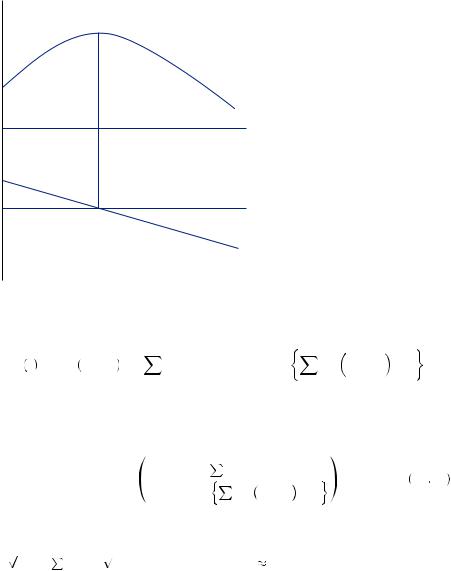
 13
13 50
50
 − 0.3, leading to a savings per week of s
  18 and ultimate utility of U
  82. In other words, people who display quasi-hyperbolic discounting according to the parameters we have specified and who are sophisticated enough to recognize the time inconsistency in their behavior would be willing to give up about a third of their savings every year just to have the commitment device that ensures that
|
|
|
|
|
360 |
|
COMMITTING AND UNCOMMITTING |
they will save. Although this is an extreme example, it illustrates how knowing that you will procrastinate in the future as well as in the present does not eliminate the welfare loss from time inconsistency. Recognizing the time inconsistency can increase your immediate well-being if commitment mechanisms are available, but there may be a heavy cost to pay for such a device.
Commitment devices have also proved to be an effective means to spur savings for retirement. Richard Thaler and Shlomo Benartzi demonstrated this when such a plan was offered to the employees of a particular manufacturing firm. Given the opportunity to commit themselves to put a fraction of future pay raises into a retirement investment, 78 percent opted to join the program, with the overwhelming majority continuing in the program through several subsequent pay raises. The retirement savings rate among participants increased from an average of 3.5 percent to 13.6 percent.
EXAMPLE 13.2 Homework Due Dates
If people recognize that they have a problem with procrastination, one result is that they may be willing to set binding deadlines for themselves. This is a form of commitment mechanism. In fact, Dan Ariely and Klaus Wertenbroch used a class of M.B.A. students to explore this possibility.
Of the students in their class, 51 were assigned three papers and told that they could be turned in at any time during the semester. The students were given the option to set whatever deadlines they wished for each of the papers. The papers would be graded such that students would lose 1 percent of their grade for every day after the deadline in which the paper had not yet been turned in. There would be no penalty for setting the deadlines later rather than earlier. In this case, time-consistent decision makers would simply decide to set the deadline at the last day of class for all three papers and turn in the papers whenever they decided to finish them. Similarly, naïve decision makers would do the same, not anticipating that they would procrastinate completing the papers. Alternatively, sophisticated decision makers may be willing to risk the penalties and set early deadlines simply to commit themselves to finish them.
In fact, the majority of students set binding deadlines: 44 days before the end of the semester for the first paper, 26 days before the end of the semester for the second paper, and 10 days before the end of the semester for the third paper. This suggests that the students understood their tendency to procrastinate and decided to use the commitment mechanism, as Odysseus did, to bind themselves to the mast. However, the authors also found that the students did not set the deadlines in a way that maximized their performance on the papers.
Another group of 48 students were given deadlines specified by the instructor. The students who did not have control over their deadlines did significantly better on the assignments, earning about 3 percentage points more than those who could choose. Perhaps we know we will be behave badly but we do not recognize the full extent of the problem.