

|
|
|
|
Budgeting and Consumption Bundles |
|
49 |
|
transaction and consumption events. Generally, this outcome has been modeled as the person maximizing the sum of consumption and transaction value functions.
Mental accounting is a collection of several theoretical concepts: budgets, accounts, reference points, value functions, consumption utility, and transaction utility. As with many behavioral models, the model makes no clear a priori predictions of behavior in many cases. Because the theory itself provides no particular guidance on how budgets or accounts are formed, in many cases, virtually any behavior could be reconciled with the general mental accounting framework. Indeed, one of the primary criticisms of behavioral economics is that by failing to make clear predictions, it might not be possible to test the proposed theory. Although it might not be possible to create a grand test of mental accounting, it is possible to test various components of the model and to discover where the particular pieces are most likely important and applicable.
Budgeting and Consumption Bundles
The use of budgeting categories creates isolated choice problems. The standard rational model supposes that all goods are considered together, implying that an overall optimum can be achieved. If a person does not have the cognitive resources to conduct the types of complicated optimization this might imply, he or she might reduce the problem into various budgets by category. So, for example, a person might have one budget for food, another for clothing, another for utilities, and so forth. In the past, people often kept separate envelopes of money for each of these budgets. More recently, people tend to use software to keep track of spending in each category.
The consumer decision problem could now be written as
max v x1, , xn k |
3 4 |
x1, , xn |
|
subject to a set of budget constraints
p1x1 + + pixi < y1, |
|
pi+1xi+1 + + pjxj < y2 |
, |
|
3 5 |
|
|
pkxk + + pnxn < yl |
|
where xs is the amount of good s the person chooses to consume, ps is the price the person pays per unit of good s, and ym is the allotted budget for category m, and where the consumer has allotted budgets to l categories over n goods.
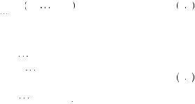
In any budget, m, the problem functions much like the standard consumer choice problem. In the category there is a budget constraint. If this constraint is binding, then the consumer chooses to consume at the point of tangency between the budget constraint and an indifference curve, given the consumption level of all other goods as pictured in Figure 3.4. Note that all of the consumption choices now depend on the reference point. We will ignore this reference point for now; however, later discussions develop this point further.
|
|
|
|
|
50 |
|
MENTAL ACCOUNTING |
x2
x2 * (ym, p1, p2 ǀ k)
FIGURE 3.4
The Consumption
Problem within a
Single Budget
Category (Holding
Consumption of All
Other Goods
Constant)
x3
x3 * ( y2 ǀ k)
FIGURE 3.5 Nonoptimality between Budgets
v(x1, x2 ǀ k)
= v(x1 * ( ym, p1, p2 ǀ k), x2 * ( ym, p1, p2 ǀ k) ǀ k)
|
x2 = ( ym –p1x1)/p2 |
x1 * ( ym, p1, p2 ǀ k) |
x1 |
v(x1, x3 ǀ k)
= v(x1 * ( y1 ǀ k), x3 * ( y2 ǀ k) ǀ k)
x3 = ( p1x1 * + p2x2 * –p1x1)/p3
x1 * ( y1 ǀ k) |
x1 |
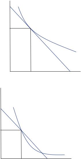
If instead we compared across budgets, we would see that the overall optimum consumption bundle is not necessarily achieved, because the budget process imposes artificial constraints. Suppose we plot two goods from separate budgets, good 1 from budget 1 and good 3 from budget 2 as pictured in Figure 3.5. With the same level of expenditure between these two goods, p1x1* y1
y1 k
k + p2x2*
 y2
y2 k
k , the consumer could purchase any bundle such that p1x1 + p3x3 < p1x1*
 y1
y1 k
k + p3x3*
 y2
y2 k
k , where we now
|
|
|
|
Budgeting and Consumption Bundles |
|
51 |
|
suppress the prices of all goods in the arguments of the consumption functions. However, the consumer did not compare these possible bundles because of the artificial budget category. Instead, the consumer found the tangency of the indifference curve to budget 1 for all items in budget 1 and then found the tangency to the indifference curve for all items in budget 3. The budget may be set such that the rational optimum is excluded. For example, the consumer might allocate less money to budget 1 than would be required to purchase the unconditional optimal bundle suggested by the standard choice problem depicted in equations 3.1 and 3.2. Further, the consumer might allocate more to budget 2 than would be suggested by the unconditional optimal bundle. In this case, the consumer will purchase less of good 1 than would be optimal and more of good 3 than would be optimal. This is the condition displayed in Figure 3.5. The indifference curve crosses the budget curve so that there are many points along the budget curve that lie to the northeast of the indifference curve, constituting the dashed portion of the budget constraint. The consumer would be better off by choosing any of these consumption points. Each of these points consists of consuming more of good 1 and less of good 3.
Thus, budgeting leads to misallocation of wealth so that the consumer could be made better off without having access to any more resources. Except in the case where the budget allocations happen to line up exactly with the amount that would be spent in the unconditional optimum, this will be the case. If particular income sources are connected with particular budgets, any variability in income leads to a further shifting of funds. For example, if money that is received as a gift is only budgeted for entertainment or for items that are considered fun, a particularly large influx of gift money will lead to overconsumption of entertainment and fun, relative to all other items. The consumer who optimizes unconditionally could instead spend much of this money on more practical items for which he or she will receive a higher marginal utility.
The consumer problem in equations 3.4 and 3.5 is solved much the same way as the standard consumer problem from Chapter 1. Now, in each budget, the consumer will consume each good until marginal utility divided by the price for each good in a budget is equal. Where  v
v x1,
x1,

 , xn
, xn k
k
 xi is the marginal utility of good i, this requires
1 |
|
|
|
|
1 |
|
|
|
|
|
|
|
|
v x1 |
*, |
, xn* k = |
|
|
|
v x1*, , xn* k , |
3 6 |
ps |
xs |
pr |
xr |
|||||||
which is the standard condition for tangency of the budget constraint with the indifference curve. Additionally, we can use the budget constraint for this particular budget to determine the amount of each good in the budget. However, the solution does not imply equality of the marginal utility divided by price for goods appearing in different budgets because they are associated with a different budget constraint. This necessarily implies that the indifference curve will cross the overall budget constraint except in the rare case that the budget is set so that the unconditional optimum described is attainable.

|
|
|
|
|
52 |
|
MENTAL ACCOUNTING |
EXAMPLE 3.3 Income Source and Spending
Since 2000, the U.S. government has cut individual income taxes several times, generally with the goal of increasing consumer spending. In each case, lowering taxes was seen as a way of combatting a sluggish economy. With lower taxes, people have more money in their pocket and thus might be willing to spend more. Nicholas Eply, Dennis Mak, and Lorraine Idson conducted an experiment whereby shoppers were intercepted in a mall and asked to recall how they had spent their rebate. The interviewer sometimes referred to the rebate as a return of “withheld income” and with other participants described it as “bonus income.” When the rebate was described as bonus income, 87 percent said they had spent it, whereas only 25 percent said they had spent it when it was described as a refund of withheld income. Further experiments confirmed that labeling income as a bonus led to greater spending than labeling it as a return of income that the participant was due.
Until 2008, the tax rebates were embodied in a one-time refund check that was sent to the taxpayer in the amount of the tax cut. For example, people who paid income tax in 2007 received a check for between $300 and $600 beginning in May 2008. A similar program in 2009 cut taxes by $400 per taxpayer. However, this cut was implemented by reducing the amount withheld from paychecks rather than in a single check. This reduction increased take-home pay by an average of $7.70 per week. Valrie Chambers and Marilyn Spencer used survey methods to determine which method of returning the money might be more effective in inducing spending. Using a sample of university students, they found that students are more likely to spend when given the money on a per-paycheck basis than when given the money as a lump sum. Students indicated that they would save around 80 percent of a lump-sum payment, whereas they would only save about 35 percent of the perpaycheck payments. This example shows how timing and the amount of the payment can influence mental accounting. Perhaps a smaller amount per week is not large enough to enter on the ledger at all and is thus more likely to be spent instead of saved.
Accounts, Integrating, or Segregating
The shape of the value function suggests that people who are experiencing multiple events will be better off when their gains are segregated and their losses are integrated (see Figure 3.3). In truth there are four possibilities for multiple events:
•If a person experiences multiple gains, x > 0 and y > 0, then concavity of the value function over gains implies that v x
x + v
+ v y
y > v
> v x + y
x + y (as in Figure 3.3). In this case, the person is better off if the events are segregated and evaluated separately.
•If a person experiences multiple losses, x < 0 and y < 0, then convexity of the value function over losses implies v x
x + v
+ v y
y < v
< v x + y
x + y (as in Figure 3.3). In this case, the person is better off if the events are integrated and evaluated jointly.
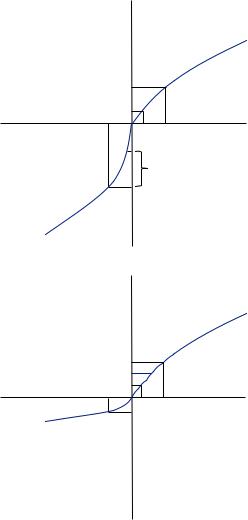
•If a person experiences a loss and a gain, x > 0 and y < 0 with x + y > 0, so that the
gain |
overwhelms |
the loss, the shape of the value function implies that |
v x |
+ v y < v x + y |
if we assume a strong form of loss aversion (Figure 3.6). |
A value function conforms to strong loss aversion if for any two positive numbers
|
|
|
|
Accounts, Integrating, or Segregating |
|
53 |
|
Utility value
v
v( x)
v(yx– y)
x − y x |
Dollar value |
v(x) + v( y) |
|
v( x) |
|
v( y) |
|
FIGURE 3.6
Integrating an Overall Gain
Utility value
v
v(x) v(x) + v( y)
v(x − y) y
x – y x |
Dollar value |
v( y) |
|
FIGURE 3.7
Integrating an Overall Gain without Strong Loss
Aversion
z1 and z2 with z1 < z2 it is always the case that vg z2
z2 − vg
− vg z1
z1 < vl
< vl z2
z2 − vl
− vl z1
z1 . This requires that a loss function always has a greater slope than the gain function a given distance from the reference point. The slope over losses near the reference point is always assumed to be steeper than the slope for gains. Further, the slope over gains is decreasing owing to diminishing marginal utility over gains. Then the decrease in utility when moving from x to x−y, given that x−y is still in the gain domain, must be less than the loss when moving from the reference point to y given strong loss aversion. In this case, the person is better off integrating the events. Without strong loss aversion, although the slope of the value function over losses is greater than for gains near the reference point, if the marginal pain from losses diminishes quickly relative to equivalent gains (shown in Figure 3.7), then the pain from the loss of y may be smaller starting from the reference point
|
|
|
|
|
54 |
|
MENTAL ACCOUNTING |
than starting from x, leading to greater total utility from segregating the events. Thus, without strong loss aversion, the problem has an ambiguous solution. We would need to specify a functional form and sizes for both events before we could determine whether one is better off integrating or segregating the events without strong loss aversion.
•If a person experiences a loss and a gain, x > 0 and y < 0 with x + y < 0, so that the loss overwhelms the gain, then we cannot determine whether integrating or seg-
regating losses makes the person better off without specifying the functional form for the value function and the size of the gains and losses. Similar to the case of mixed outcomes leading to an overall gain, we could impose restrictions that would allow us to determine the outcome. In this case, we would need to require that for any two positive numbers z1 and z2 with z1 < z2 it is always the case that vg z2
z2 − vg
− vg z1
z1 > vl
> vl z2
z2 − vl
− vl z1
z1 . However, this violates the basic assumptions of loss aversion, requiring that the slope of the gain function be greater at the reference point than the slope of the loss function is. Thus, we ignore this case. However, as a rule, if gains are very small relative to the losses, they should be segregated. Again this results because the slope of the value function over losses is relatively small farther away from the reference point. Thus, the increase in utility from a small gain starting from a point very far to the left of the reference point will be small relative to the same gain beginning at the reference point.
The early literature on mental accounting supposed that people would be motivated to group events in order to make themselves feel better off. If this were the case, people who had faced multiple gains would choose to segregate them to maximize their utility. Someone facing multiple losses would choose to integrate them to maximize utility. Further, people who lose an item that was recently given to them as a gift will be better off considering this the elimination of a gain rather than an outright loss. This is due to the steeper slope of the value function over losses than gains. This theory has been called hedonic editing.
However, initial research by Eric Johnson and Richard Thaler suggests that people do not engage in hedonic editing. Johnson and Thaler tested the hedonic editing hypothesis by offering subjects the choice between gains and losses spaced over different time periods. The idea was that offering a pair of losses or gains spaced farther apart in time might make it easier for the subject to segregate the outcomes. Johnson and Thaler found that subjects preferred gains to be spread out and they also preferred losses to be spread over time. Thus, people prefer to spread all changes over time, whether positive or negative.
Prior research by Richard Thaler had asked subjects several questions regarding outcomes that were described in ways that were intentionally worded to integrate or separate outcomes. For example, one question asked whether a man who received notice that he owed an unexpected additional $150 on his federal income taxes would feel better or worse than a man who received notice that he owed $100 in federal income taxes and another notice that he owed $50 in state income taxes. Among this set of questions, participants showed a clear preference for segregating gains and integrating losses. When the wording of a question, independent of the actual outcomes, influences