


 1
1  , then betweenness is satis


 ,
, 
 is a standard utility of wealth function, and
 constitutes some function used to weight the probabilities associated with particular outcomes. To derive indifference curves, consider all points
 such that
 33
33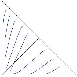
|
|
|
|
|
236 |
|
DECISION UNDER RISK AND UNCERTAINTY |
which, because outcomes and the functions u and v are fixed, yields an equation of the standard linear format p1c1 + p2c2 + c3 = 0. To see that the slopes of the indifference curves may be different, note that k is a parameter of the constants c1, c2 and c3. Thus, the slope depends upon the level of utility indicated by the indifference curve.
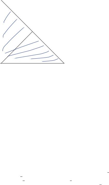
Several have noted that the weighted utility model does fit the data in the triangle significantly better than the expected utility model. However, others have noted that there is significant evidence that betweenness is violated. Colin Camerer and Tek-Hua Ho find that in laboratory settings, people show clear evidence of nonlinear indifference curves. Interestingly, however, the shape of the indifference curves depends substantially on the types of gambles presented. In particular, gambles that involve losses generate a very different pattern of indifference curves from those generated by gambles involving gains.
The Shape of Indifference Curves
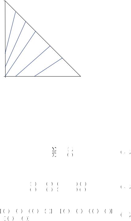
By repeatedly asking people to choose between pairs of gambles representing different points in the Marschak–Machina triangle, experimental economists have discovered many regularities in the shapes of these indifference curves. Figure 9.6 provides an example of the general shapes of indifference curves found in laboratory experiments for gambles involving gains. In general, the curves are steeper than the 45-degree line in the northwest portion of the triangle, and they are flatter than the 45-degree line in the southeast portion of the triangle. The curves display significant fanning out around both the vertical and horizontal axes. However, the curves are close to parallel in the center of the triangle. There is some weak evidence that curves actually fan in around the hypotenuse of the triangle. Thus, the places where violations of expected utility are most likely to occur are near the edges of the triangle, where very large and very small probabilities are involved. Interestingly, when gambles with losses are examined, the indifference curves appear to be
|
Probability of highest value |
FIGURE 9.6 |
|
Indifference Curves in |
|
the Triangle for Gam- |
|
bles Involving Gains |
Probability of lowest value |


 , which maps probabilities onto the unit interval. Generally
 is thought to be an increasing function of the true probability, with


 is a concave function when
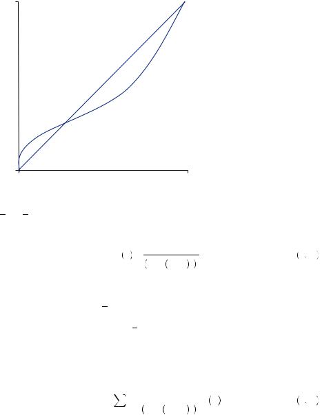
|
|
|
|
|
238 |
|
DECISION UNDER RISK AND UNCERTAINTY |
1
Probability weight
FIGURE 9.8 |
0 |
|
|
A Typical Probability |
|
1 |
|
Weighting Function |
0 |
Probability p |
|
|
|
p = π p
p ) is believed to be smaller than 0.5. One commonly used functional form for a probability weighting function is given by
π p = |
pγ |
|
pγ + 1 − p γ 1γ . |
9 34 |
This function has the same inverted s-shape as the function presented in Figure 9.8. Probability weights imply subadditivity under the right circumstances (for example, if all probabilities are larger than p) and could thus explain the certainty effect. Alternatively, probability weighting would imply superadditivity (probabilities sum to greater than 1) if all outcomes had probability below p, suggesting uncertain outcomes would be unduly preferred to certain outcomes in some cases.
Finally, probability weighting functions make preferences a nonlinear function of the probabilities. For example, using the probability weighting function above, the value of a gamble would be given by
V = |
n |
|
piγ |
|
U xi . |
9 35 |
i = 1 |
γ |
|
1 |
|||
|
1 − pi |
γ |
|
|||
|
|
pi + |
γ |
|
||
|
|
|
|
|
||
Given the highly nonlinear nature of the function with respect to the probabilities, the indifference curves are also necessarily very nonlinear, potentially allowing the possibility of explaining some of the fanning out or fanning in of the indifference curves. In particular, if the slope of the probability weighting function only changes substantially for very high probabilities or very low probabilities, that might explain why the indifference curves in the triangle only display changes in slope near the edges of the triangle (or where some probability is necessarily low and another is necessarily high).