


|
|
|
|
|
126 |
|
BRACKETING DECISIONS |
Much like the framing effects discussed in previous chapters, how decisions are grouped together can have a tremendous impact on which outcomes look most attractive. Although few in the position of needing to work on a substantial class project in the next 48 hours would choose to play video games for several hours straight before beginning the project, many might make several individual decisions to play for 20 minutes at a time. Further, whereas a single investment choice might sound prohibitively risky, a group of many choices each bearing the same risk might sound very attractive. Bracketing or choice bracketing refers to how choices are grouped together. Often choices are grouped naturally by their placement in time. For example, one generally decides on what to have for breakfast before deciding on what to have for lunch or dinner. Nonetheless, decisions regarding the size and content of breakfast can severely affect what may practically be eaten for lunch. Once you have had an especially large lunch, you might feel uncomfortable having a particularly heavy dinner in addition.
Decision bracketing is closely related to hedonic editing or framing. However, hedonic editing and framing deal only with how people evaluate events (valuing them more or less), whereas choice bracketing deals directly with how the decisions themselves are made (which tradeoffs or variables are considered when making the choice). Choice bracketing has implications both for risky and riskless choice. However, discussing risky choice requires some review of rational choice under uncertainty, hence the placement of this chapter in the Information and Uncertainty section of the book. We review rational models of multiple decisions as well as the most widely accepted rational model of decision under risk: expected utility theory. This model is covered in greater detail in Chapter 9, including its axiomatic foundation (i.e., why we consider it rational).
Multiple Rational Choice with Certainty and Uncertainty
Rational choice theory generally supposes that a person makes a single decision to purchase a consumption bundle rather than making a series of individual purchase decisions for each item in the bundle. This abstraction is considered necessary in order to allow the theory to address the wide variety of purchasing decisions that people make. Truly, very few purchasing decisions are made simultaneously. Consider, for example, that we wish to model food consumption for lunch and dinner of a particular day. For simplicity, suppose that there are only two items that can be purchased for lunch: either one peanut butter sandwich, x1, or one ham sandwich, x2. Also, suppose there are only two items that can be purchased for dinner, either one steak, y1, or one plate of pasta, y2. Further, assume that the person must eat both lunch and dinner (so not consuming is not an option) and that both lunch options and both dinner options cost exactly the same amount. If the person were to make a single decision at lunchtime regarding consumption of both lunch and dinner, we may model the individual problem as
max U x, y . 6 1
1
x x1,x2 , y y1,y2
|
|
|
|
Multiple Rational Choice with Certainty and Uncertainty |
|
127 |
|
In this case there are four possible consumption bundles of lunch and dinner. Suppose that the diner’s preferences could be represented as U x1, y1
 > U
> U x2, y2
 > U
> U x2, y1
 > U
> U x1, y2
 , so that the diner most enjoys eating a peanut butter sandwich for lunch and a steak for dinner and least enjoys eating a peanut butter sandwich for lunch with a plate of pasta for dinner. If taken all together, this diner will always choose the most-preferred bundle.
Suppose instead the diner made the choices sequentially, so that lunch is determined around noon and dinner is determined in the evening. If the diner is certain of the options that will be available at the time of the dinner decision when making the lunch decision, then iterating these decisions should have no impact on the chosen consumption bundle. At lunchtime, the diner would still consider which lunch would give her the greatest utility in combination with the two possible dinners and would decide on the peanut butter sandwich, intending on having the steak. When dinnertime arrives, given the previous consumption of the peanut butter sandwich, the steak will seem more attractive
and thus the diner will fulfill her plan. We can write this iterated decision as |
|
|
max |
max U x, y , |
6 2 |
x x1,x2 |
y y1,y2 |
|
which will always yield mathematical results that are identical to equation 6.1. To see this, consider solving equation 6.2 sequentially beginning with the expression in the braces (like backward induction from game theory). In this case, one will choose y to maximize utility given x and thus will choose y1 if x = x1 and y2 if x = x2. After solving for y as a function of x, we must evaluate the maximization over x. In this case, the diner is choosing between  x1, y1
 and
and  x2, y2
 , which results in a choice of
  x1, y1
 . Thus, in the rational model, if the diner knows all the choices she will face in the future at each point, segmenting or sequencing decisions should not have any impact on the final decision. This result is called segmentation independence. Under all rational models, the division or segmenting of decisions should not affect the final decision so long as the availability of decisions is known and certain beforehand.
A version of segmentation independence holds if the outcomes from choices are unknown when employing a rational model of choice under risk. The commonly accepted rational model of decision under risk is the expected utility model. For now we introduce the expected utility model briefly. In later chapters, we describe the foundation for expected utility and why it is considered a rational model.
The expected utility model supposes that a person maximizes the expectation (or mean) of utility. For example, consider a gamble that yields $100 with probability 1/2 and − $100 with probability 1/2. Probability gives us the percentage of times an event will happen if we could repeat the experiment an infinite number of times. In this case, the expected value of the gamble is found by summing each outcome multiplied by the percentage of times that outcome would occur if we repeat the experiment a large number of times, E π
π = 0.5
= 0.5  100 − 0.5
  100 = 0. This is essentially the average value we would expect given a large sample of observed outcomes from this gamble. Thus on average, one gains and loses nothing by taking this gamble. Alternatively, suppose that the person has a utility of money function u
 π
π , with u
 100
100 = 1, u
 − 100
− 100 = − 2, and that u
 0
0 = 0. Then the expectation of the utility function is found by multiplying the
128
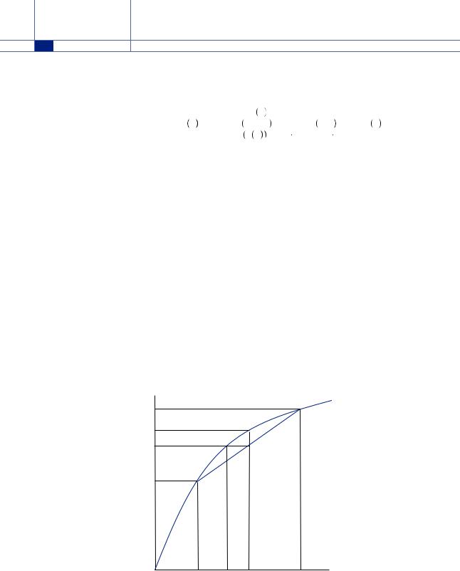
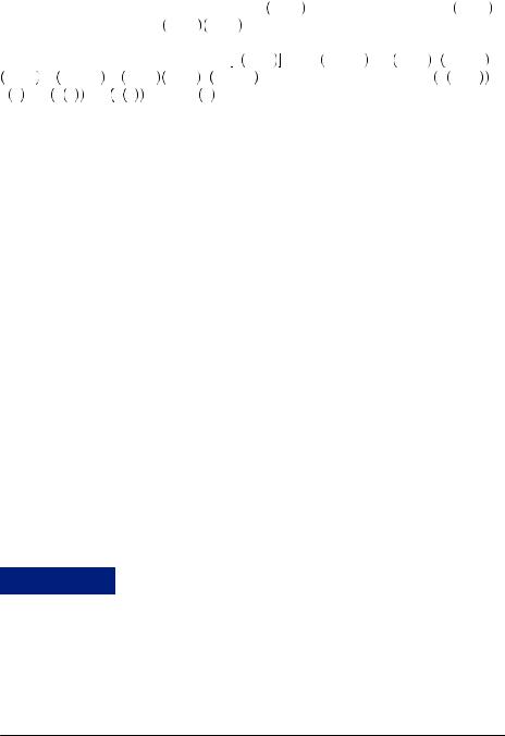
FIGURE 6.1
Risk Aversion under Expected Utility Theory
BRACKETING DECISIONS
probability of each outcome by the utility of that outcome, E u
u π
π = 0.5
= 0.5  u
u 100
100 + 0.5
+ 0.5  u
u − 100
− 100 = 0.5
= 0.5  1 − 0.5
  2 = − 0.5. The expected utility of the gamble is below zero in this case (because the loss of utility from losing $100 is greater than the gain in utility from gaining $100), and thus the person would prefer to refuse the gamble and obtain the
utility of no change in wealth, u 0 |
= 0. If instead each dollar yielded a constant rate |
|
of utility, say u 1 = 1, then u − 100 |
= − 100, u 100 |
= 100, u 0 = 0. In this case, the |
expected utility is given by E u π |
= 0.5 100 − 0.5 |
100 = 0. Thus, the person would |
be indifferent between taking the gamble or not.
Consider Figure 6.1, which depicts a person’s evaluation of a gamble with probability of 0.5 that the person obtains x1 and probability 0.5 that the person obtains x2, where x1 and x2 are amounts of money. The expected payoff from this gamble,
E x
x = 0.5x1 + 0.5x2, is represented by the location on the x axis that is exactly equidistant from x1 and x2. If the person could obtain the expected value of the gamble with certainty, she would obtain u
 E
E x
x , as depicted on the y axis. Instead, she values the gamble according to its expected utility, given by E
 u
u x
x = 0.5u
 x1
x1 + 0.5u
 x2
x2 , which is the location on the y axis that is exactly equidistant from u
 x1
x1 and u
and u x2
x2 . Note the shape of the utility function in Figure 6.1 is concave, displaying diminishing marginal utility of wealth. This means that the slope of the utility function between E
 x
x and x2 is smaller than between x1 and E
 x
x , leading the midway point between u
 x1
x1 and u
and u x2
x2 to fall below u
 E
E x
x . Thus, the gambler would prefer to have the expected value of the gamble with certainty than to take the gamble and obtain the resulting expected utility.
Further, we can define the certainty equivalent as the amount of money with certainty that yields the same level of utility as the expected utility of the gamble, or 
 = 0.5u
 x1
x1 + 0.5u
 x2
x2 , where xCE is the certainty equivalent. In Figure 6.1, the certainty equivalent falls below the expected value of the gamble, reflecting that the person is willing to give up some amount of money on average in return for certainty. In general, if a person is willing to take a reduced expected value to obtain certainty, we call the person risk averse.
u(x) u(x2)
u(E(x))
E(u(x))
u(x1)
x1 |
xCE E(x) |
x2 |
x |
|
|
|
|
Multiple Rational Choice with Certainty and Uncertainty |
|
129 |
|
Under the expected utility model, diminishing marginal utility of wealth, as displayed by a concave utility function, implies risk aversion. Diminishing marginal utility of wealth simply requires that the next dollar provides less utility to a wealthy person than to a poor one. Consider a more general gamble with α probability of obtaining x1 and  1 − α
1 − α probability of obtaining x2. The person displays risk aversion if for any two amounts of money x1 and x2, the utility function is such that
u αx1 + 1 − α x2 > αu x1 + 1 − α u x2 , |
6 3 |
or if the expected utility from the gamble is lower than the utility of the expected value. This necessarily implies that the certainty equivalent is less than the expected value of the gamble (because it yields lower utility). Because 0 < α < 1,
u αx1 + 1 − α x2 = αu ax1 + 1 − α x2 + 1 − α u αx1 + 1 − α x2 . |
6 4 |
|||||
Substituting equation 6.4 into equation 6.3 yields |
|
|||||
α u αx1 + 1 − α x2 − u x1 > 1 − α u x2 − u αx1 + 1 − α x2 . |
6 5 |
|||||
If we suppose that x2 > x1, then dividing |
both sides of (6.4) by α 1 − α |
x2 − x1 , |
||||
obtains |
|
|
|
|
||
|
u αx1 + 1 − α x2 − u x1 |
> |
u x2 − u αx1 + 1 − α x2 |
|
6 6 |
|
|
α x2 − x1 |
|||||
|
1 − α x2 − x1 |
|
|
|||
or adding and subtracting x2 from the denominator of the right side and rearranging the denominator of both sides yields
u αx1 + 1 − α x2 − u x1 |
> |
u x2 |
− u αx1 + 1 − α x2 |
. |
6 7 |
αx1 + 1 − α x2 − x1 |
|
|
|||
|
x2 − αx1 + 1 − α x2 |
|
|||
Note that the terms on both sides of the equation are analogues of the slope or derivative of the utility function, having the familiar form of rise over run. The left side term is the slope of the utility function between x1 and αx1 +  1 − α
1 − α x2, and the slope of the right side term is the slope of the utility function between x2 and αx1 +
  1 − α
1 − α x2. Thus, equation 6.7 simply says that the slope over the upper portion of the curve is smaller than the one over the lower portion of the curve. Reflecting on equation 6.3, the condition in this equation is the general condition for concavity of a function or diminishing marginal utility of payouts. Thus in general, a concave utility function implies risk aversion under expected utility theory.
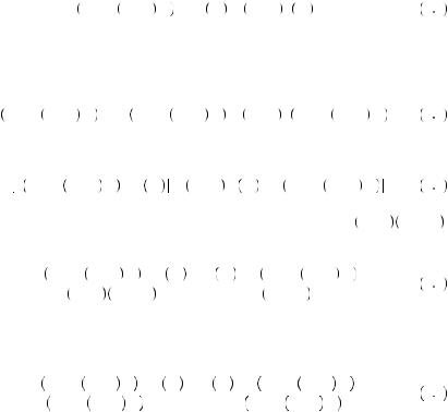
If instead the utility function is linear, u x
x = ϕx, where ϕ is a scalar constant, the utility function implies that risk itself does not matter. This case is depicted in Figure 6.2. In this case, the slope of the utility function is constant everywhere. Thus, a dollar means as much to the person no matter what her starting wealth. In this case, the analogue to equation 6.7 requires that
|
|
|
|
|
130 |
|
BRACKETING DECISIONS |
FIGURE 6.2
Risk Neutrality under Expected Utility Theory
u(x) u(x2)
u(E(x)) = E(u(x))
u(x1)
x1 |
E(x) = xCE |
x2 |
x |
|
u αx1 + 1 − α x2 − u x1 |
= |
u x2 − u αx1 + 1 − α x2 |
= ϕ. |
6 8 |
αx1 + 1 − α x2 − x1 |
|
||||
|
|
x2 − αx1 + 1 − α x2 |
|
||
Also, the expected utility can be calculated as |
|
||||
|
E u x = αϕx1 + 1 − α ϕx2 = ϕ αx1 + 1 − α x2 = u E x . |
6 9 |
|||
Thus, no matter how much risk is involved, the expected utility of the gamble equals the utility of the expected value of the gamble if the utility function is linear. If the person is risk neutral, the expected value of the gamble always equals the certainty equivalent. In the expected utility model, a risk-neutral decision maker is always represented by a linear utility function.
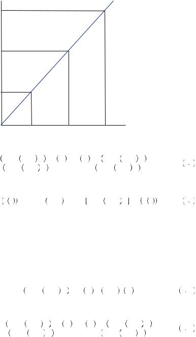
Finally, consider the case of a convex utility function. In this case, the person is risk loving, meaning she prefers a gamble to its expected value. Thus, in this case we reverse the relationship in equation 6.3,
u αx1 + 1 − α x2 < αu x1 + 1 − α u x2 , |
6 10 |
which, after following the same steps as before, yields
u αx1 + 1 − α x2 − u x1 |
< |
u x2 |
− u αx1 + 1 − α x2 |
. |
6 11 |
αx1 + 1 − α x2 − x1 |
|
|
|||
|
x2 − αx1 + 1 − α x2 |
|
|||
Thus, the slope above the expected payout from the gamble must be larger than the slope below the expected payout of the gamble. This possibility is displayed in Figure 6.3. Here, the certainty equivalent is above the expected value of the gamble. As well, the
|
|
|
|
Multiple Rational Choice with Certainty and Uncertainty |
|
131 |
|
u(x) u(x2)
E(u(x))
u(E(x))
u(x1)
|
|
|
FIGURE 6.3 |
x1 |
E(x) xCE |
x2 |
x Risk Loving under Expected Utility Theory |
expected utility of the gamble is above the utility of the expected value of the gamble. In general, a convex utility function implies risk-loving behavior.
Part of the long love affair between economists and the expected utility model is due to the model’s simplicity. All risk preferences are completely captured in the curvature of the utility function, which represents how money is valued over various levels of wealth. If one has a concave utility function, one is willing to pay less than the expected value of winning the lottery (a truly small number) for a lottery ticket, because the value of the ten millionth dollar (and every dollar above the initial outlay) one could possibly win is much smaller than the value of the dollar one must pay to buy it. Alternatively, if one has a convex utility function, one would be willing to pay more than the expected value of the lottery ticket, because the value of every dollar one could win above the amount one must pay for the ticket is worth more to one than the dollar one would pay to buy it.
Risk aversion is commonly measured using coefficients of absolute or relative risk aversion. The coefficient of absolute risk aversion is given by RA = − u″ w
w u
u w
w , where u
 w
w is the marginal utility of wealth and u
 w
w is the slope of the marginal utility of wealth curve evaluated at w. The coefficient RA is a simple measure of concavity of the utility function: the more concave, the larger the value RA. The higher the level of absolute risk aversion, the less willing to take any particular gamble the decision maker will be. A closely related measure of risk aversion is relative risk aversion, given by RR = wRA, where w is wealth. The higher the degree of relative risk aversion, the less willing to risk a particular portion of her wealth the decision maker will be. Generally, economists suppose that relative risk aversion falls between 1 and 3.
Now, with the basic tools of expected utility theory, consider the person who must decide whether to take either or both of two gambles. One gamble yields x1 with probability α and x2 with probability  1 − α
1 − α . The second gamble yields y1 with probability β and y2 with probability
  1 − β
1 − β . For simplicity, let us suppose that the gambles are independent, so that the outcome of one gamble does not depend upon the outcome
|
|
|
|
|
|
|
|
132 |
|
BRACKETING DECISIONS |
|
|
|
|
|
of another. In this case, taking both gambles would result in a gamble that yields x1 + y1 |
||||
|
|
with probability αβ, x1 + y2 with probability α 1 − β , x2 + y1 with probability 1 − α β, |
||||
|
|
and x2 + y2 with probability 1 − α 1 − β . We call this a compound gamble because it |
||||
|
|
is a gamble composed of two other gambles combined. Thus the expected utility of |
||||
|
|
taking both |
gambles together is E u x + y |
= αβu x1 + y1 + α 1 − β u x1 + y2 |
+ |
|
|
|
|
1 − α βu x2 + y1 + 1 − α 1 − β u x2 + y2 . |
Suppose for now that E u x + y |
> |
|
|
|
u 0 > E u y |
> E u x , where u 0 is the utility of refusing both gambles. As with the |
|||
choice problems in equations 6.1 and 6.2, the choice between taking and not taking each gamble is independent of segmentation. In other words, if asked to choose simultaneously, the person in this example would choose both gambles. If asked to first choose whether to take x, and then whether to take y, the person should make the same decision so long as she understands that both choices will be offered to her. She would consider y to be beneficial given x is chosen but not if x is rejected. Thus, the choice is either x and y or no gambles. In this case she would choose both.
Paul Samuelson observed that this segmentation independence has some implications for choice between an individual risk and multiple risks. Suppose that someone is unwilling to take a gamble x because she considers the gamble to be too risky. Then it is very unlikely that she would be willing to take two identical gambles x. In particular, suppose that the maximum she could gain or lose by taking gamble x is $k. Because risk preferences are determined by a utility of money function, a person’s behavior depends on her level of wealth. Suppose the person has initial wealth w. If her risk preferences are such that she is unwilling to take the bet given any wealth level in the range of wealth  w −
w −  n − 1
n − 1 k, w +
  n − 1
n − 1 k
k , where n is some positive integer, then she will be unwilling to take a combination of n identical gambles x.1 The segmenting works just as before. If someone is unwilling to take the gamble x over a range of wealth
  w − k, w + k
 , then suppose she somehow was given the one gamble x against her will. She would still be unwilling to take the second bet no matter the outcome of the first gamble because wealth still falls within the relevant range. If the person would reject each individually given sequential decision, then she would reject both jointly by segmentation independence. Thus, if you are unwilling to take a 50 percent chance of winning $200 and a 50 percent chance of losing $100, and this preference would persist if your wealth shifted by $2,000, you should be unwilling to take 10 such chances together.
EXAMPLE 6.1 Paul Samuelson and His Colleague
Out at lunch with his colleagues one day, Paul Samuelson proposed a bet to each person at the table. He would pay them $200 if they could predict the result of a single coin toss, and if not they would pay him $100. One of his colleagues, whom Samuelson describes as a distinguished scholar with no claim to advanced mathematical skills, answered, “I won’t bet because I would feel the $100 loss more than the $200 gain. But I will take
1 Actually, the required range of wealth is much smaller and could be rather negligible. However, the intuition is easiest to explain with the given range. In truth, the range need only cover the loss between current wealth and the certainty equivalent of the gamble multiplied by n.