d

λ = 161.3 mm, l = 0.44 λ, d = 0.006 λ, w = 0.003 λ, a = 0.225 λ, h = 0.056 λ, s = 0.006 λ

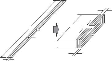
Figure 10.3 Folded loop antenna element.

10.3.2Antenna structure

A folded loop introduced here is the antenna previously described in 8.1.2 (2)-2b, which is essentially a two-wire transmission line, folded at about a quarter-wavelength to form an equivalent half-wave folded dipole, and yet appears as a one-wavelength loop antenna, from which the antenna is referred to as a folded loop. The element taken as an example here is made of thin copper wire with a diameter of 0.5 mm. The folded wire element forms a very thin (d λ) rectangular loop that is considered as a folded dipole as shown in Figure 10.3. The length l of the folded loop is about 1/2 wavelength at the center frequency f0 which equivalently corresponds to a half-wavelength folded dipole and at the same time to a one-wavelength loop. By selecting the two-wire transmission line parameters, the antenna input impedance can be adjusted flexibly, since the reactance of the transmission line can be adjusted by selecting the length and the width of the wires and the distance between the two lines. This is the important feature of this antenna, which is constituted by applying the integration technology.

Figure 10.4 shows the configuration of the antenna element and the finite GP that represents a shielding plate when it is used in the handset. The antenna element is placed very closely to the rectangular GP, which has the perimeter of about two wavelengths. Both unbalanced and balanced type of feed are considered here as Figure 10.4(a) and (b) show. The unbalanced feed is tested only to confirm the effectiveness of the unbalanced feed for the folded loop, as the folded loop of a half wavelength has performance similar to the balanced system. The antenna element is fed by either a coaxial cable (Figure 10.4(a)) or a parallel line (Figure 10.4(b)). In the experiment, a semi-rigid coaxial cable with a diameter of 0.011λ is used and the load of a 50 : 50 chip balun is used for the balanced system. The center frequency f0 is 1860 MHz.

In the numerical analysis, various types of electromagnetic simulators are applied based on the method of moments (MoM) [23], finite-difference time-domain (FDTD) method [24], finite element method (FEM) [25], and finite integration method (FIM) [26].

Coaxial cable (0.011λφ)

Chip balun

Figure 10.4 Antenna structure: (a) unbalanced feed and (b) balanced feed.

The electromagnetic simulators including antenna and propagation problems are widely used nowadays as the computational capacities of personal computers and workstations have become adequate. However, as the simulators are not perfect for analyzing antenna problems, users need to have experience with the simulators and be acquainted with their individual characteristics.

Figure 10.5 shows the feeding method of each electromagnetic simulator. In the MoM simulation, since the models are divided into small cells automatically, the standard frequency of the division employs 2500 MHz, higher than the required frequency. To confirm the convergence, the results of four models which have divisions from 10 to 30 cells per wavelength (i.e., size ranging from 0.03λ to 0.1λ) are compared and discussed. When the number of cells per wavelength is 20, the numbers of total cells of unbalanced-fed and balanced-fed models are 509 and 458, respectively. The feed type used in simulation is horizontal port which is called “Extension for MMIC” (Monolithic Microwave Integrated Circuit). A length of the edge cell is one tenth of the feed line’s width empirically.

In the FDTD simulator, models are divided into non-uniform meshing of 0.5 to 4 mm. Around the feed point the structure is divided into minimum cells of 0.5 mm, while the part where there is no influence in the calculation is divided into larger cells to reduce the total number of cells. The total number of cells is 49 140 and all parts of models use Perfect Matching Layer, which is referred to as PML, as absorbing boundary conditions. The feed type used in the simulation is “Coaxial Port” and “Gap Port.”

In the FEM simulator, models are divided by using automatic adaptive mesh. Therefore, the model of the handset, which is used here as an example, is divided into small cells effectively. The total number of cells is 389 160. The large models such as human

head or hand model are divided into the larger cells by using manual mesh to reduce the number of total cells. The feed type used in the simulation is a coaxial port.

10.3.3Analytical results

Figure 10.6 shows the simulated current distribution on the GP at the center frequency by using the MoM simulator, where (a) shows for the case of an unbalanced system and

(b) shows for the case of a balanced system. Since the antenna element is placed on the GP so as to make the system structure symmetrical with respect to the center of the GP (the x–z plane) the current distributions on the GP obviously become symmetrical. The figure illustrates the current distributions on the GP only, not including those of the antenna element, and the amplitude of currents is shown with gray shading. In the figure, the fainter shading indicates greater current flow while the darker color part indicates smaller current flow. The antenna element is located on the left side of the GP.

As shown in the figure, while only a slight difference is seen around the feed point between the current distributions in both unbalanced and balanced system, at other points they have almost the same amplitudes. For the unbalanced system, the current