9.3Practice of measurement

Figure 9.18 Radiation resistance and inverse of input reactance.

Stability of the instrument is also important because, if the instrument is not stable enough, errors due to fluctuation in the measurement system become involved in the measured results. For instance, when a small impedance of an ESA, e.g., about 1 is measured, stability of the instrument must be high enough to determine one-tenth of 1 or so. The results obtained by the measurement with an unstable instrument are meaningless.

The bandwidth f is the range of frequencies on either side of a center frequency, at which the antenna characteristics such as impedance, gain, radiation efficiency, and so forth, are within an acceptable range of those at the center frequency. For narrow band

where f1 and f2, respectively, are the higher and the lower frequencies, at which the power declines 3 dB from the maximum and f0 is the center frequency of the bandwidth f. This B is referred to as the relative bandwidth and is practically used instead of the

bandwidth f. The center frequency f0 is given by

Quality factor Q can be used instead of the relative bandwidth B when the bandwidth f is narrow (B < 10 %),

9.3.2Radiation patterns and gain

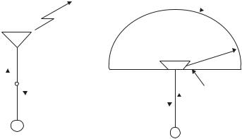
The radiation field for an antenna consists of a near-field region close to the antenna and a far-field region further away from the antenna. Here, measurement for the far-field radiation pattern is presented. The far-field region can be defined by calculating the phase error due to the finite size of the antenna. Figure 9.19 shows the difference in the path length from the observation point to the center of the antenna system, and to the end of the antenna. This path length difference can be translated into a phase difference

R′

D

R

Figure 9.19 Definition of the far field.

as indicated by the equation:

For the phase error to be less than π /8, the distance R from the antenna must be such that:

The above equation is often used to define the far-field distance for antennas.

9.3.3Efficiency measurement

There are three typical methods to determine the antenna efficiency: pattern integration method, Q-factor method, and Wheeler method [8].

The pattern integral method determines Prad from the integration of the radiation pattern intensity, which is obtained from the far-field measurement. While pattern integration is considered the most accurate method available, especially when the absolute efficiency of an antenna is desired, it usually takes a rather long time, because it needs to measure radiation patterns and to perform integration of the radiation patterns over a spherical surface completely enclosing the antenna.

On the contrary, Q-factor and Wheeler methods have the advantage of being quick and easy to employ, as compared to the pattern integration method. These two methods relate the antenna efficiency to the input impedance rather than the far-field pattern integration. These two methods have the advantage that the measurement does not require any particular system, but can employ ordinary methods, and also can be performed in ordinary laboratory rooms. However, there is a trade-off between the accuracy and ease of the measurement because the accuracy of the antenna efficiency obtained by these two methods is relatively lower than by the pattern integration method.

The Q-factor method is based on a measurement of two antenna Q values, one is the QRL of the test antenna and another is the QR of an ideal antenna. QRL can be determined by measuring the impedance of the test antenna. QR can be determined from calculation based on Chu’s theory. If the Q of an antenna is high, it can be interpreted as the reciprocal of the relative bandwidth B. The B can be known from the impedance–frequency characteristics. B is defined as the bandwidth for the half-power

Wheeler cap

frequencies that occur for a power reflection coefficient of 0.5 (VSWR = 5.83). Because of the inherent difficulty in determining QR, the Wheeler method is recommended because it is simpler in practice.

In the Wheeler method (Figure 9.20), the antenna resistance is measured in two ways: Rin of an antenna reradiating into free space and Rloss of an antenna placed within a Wheeler cap, which eliminates radiation from the antenna. By using these two resistances Rloss and Rin, Rrad can be found, since Rin = Rrad + Rloss. Then the efficiency η is calculated from

The dimension of a cap is recommended to be about λ/2π , although there have been no exact theories to prove this idea. By experimental studies, it is understood that there seems to be no severe limitation in the cap size unless it greatly exceeds λ/2π . It was also confirmed that the radius of the Wheeler cap can be as large as 10 times a radian length, granted that resonance and interference of the Wheeler cap on the frequency characteristics of the testing antenna can be avoided [9]. For the shape of a cap, other types than a sphere such as a cube, a rectangular solid, can be used. The shape somehow depends on the size and type of test antennas. For a thin, short monopole, both hemispheric and cubic shapes can be used. A cubic shape seems to be better for antennas such as an inverted-F antenna, because it has an element parallel to the sides of the cap, and the distance between the antenna element and the cap can be made nearly equal; thereby, variation in the antenna current is made small after the cap covers the antenna.

In any case, care must be observed for the resonance or anti-resonance of the antenna, cap, or both. Note that the principle of the Wheeler method is based on the measurement of the series resistance or the parallel conductance. At or near resonance or anti-resonance frequencies, resistance or conductance becomes very low or approaches an infinitely large value and no consistency in the measured values can be expected.

Without cap

Spherical cap

Cubic cap

Real

Imaginary

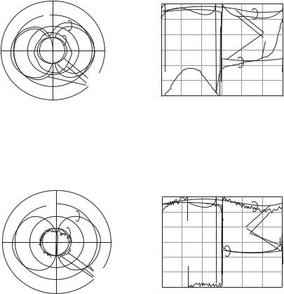
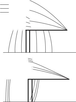
Figure 9.21 Current distributions on inverted F antenna element (800 MHz).

The inner surface of a cap should be plated to reduce the ohmic loss. Usually, the interaction of the cap surface current with the antenna current is ignored because it can be assumed to be very small. However, it may become an appreciable value when the antenna element approaches the inner surface of the cap because the cap surface current may interact with antenna current. Then the cap surface loss becomes included in the antenna loss. Plating the cap surface with gold is best.

Another problem in the Wheeler method lies in an assumption that the antenna current is not changed by the presence of the Wheeler cap. This is not really true. Figure 9.21 shows that the antenna current of an inverted-F antenna varies due to a Wheeler cap [10]. Variation of the current depends on the shape and the size of the Wheeler cap as well as the type and the size of the antenna. Errors in the measurement are greatly increased, especially at the frequency of resonance or anti-resonance, which depend on the type and size of the antenna as well as the shape and size of the Wheeler cap.

Radiation efficiency of a small antenna located in some complicated environment can be evaluated in the reverberation chamber [11]. The radiation efficiency, for instance, of a small built-in antenna installed in a small handset, which is held by an operator, differs from that of a small antenna located in free space, because the radiated power from the handset is varied by the environmental materials. In addition, in practical operation, especially in an urban field, the incident or generated field by the antenna is not uniform, but rather random, including cross-polarized radio waves, due to the environmental conditions in the wave propagation path. In the reverberation chamber,

388Evaluation of small antenna performance

radiation efficiency can be evaluated in an environment, where non-uniform field, which equivalently corresponds to the field around the antenna, can be easily produced. In the evaluation of the radiation efficiency, the radiation power from the handset is measured in the reverberation chamber and the efficiency is determined by taking a ratio of the radiated power to the input power to the antenna [12].

Input impedance of a very small antenna located near lossy materials can also be evaluated in the reverberation chamber [13]. An example is again a small built-in antenna installed in a small handset and a lossy human operator holds the handset.

References

[1]T. Fukasawa, K. Shimomura, and M. Ohtsuka, Accurate Measurement Method for Characteristics of an Antenna on a Portable Telephone (in Japanese), IEICE Transactions on Communications, vol. J86-B, September 2003, no. 9, pp. 1895–1905.

[2]C. Icheln, J. Krogerus, and P. Vainikainen, Use of Balun Chokes in Small-Antenna Radiation Measurements, IEEE Transactions on Instrumentation and Measurement, vol. 53, April 2004, no. 2, pp. 498–506.

[3]C. A. Balanis, Antenna Theory: Analysis and Design, 2nd edn., John Wiley and Sons, 1997.

[4]H. Garn, M. Buchmayr, and W. Mullner, Tracing Antenna Factors of Precision Dipoles to Basic Quantities, IEEE Transactions on Electromagnetic Compatibility, vol. 40, November 1998, no. 4, pp. 297–310.

[5]H. Saito, I. Nagano, S. Yagitani, and H. Haruki, Radiation Characteristics of Antenna for a Small Radio Terminal in Vicinity of a Human Body (in Japanese), IEICE Transactions on Communications, vol. J83-B, October 2000, no. 10, pp. 1437–1445.

[6]T. Uno and S. Adachi, Range Distance Requirements for Large Antenna Measurements,

IEEE Transactions on Antennas and Propagation, vol. 37, June 1989, no. 6, pp. 707–720.

[7]I. Ida, T. Sekizawa, H. Yoshimura, and K. Ito, Dependence of the efficiency-bandwidth product of small dielectric loaded antennas on the permittivity, Proceedings of ISAP 2000, vol. 1, pp. 61–64.

[8]E. D. Newman, P. Bohley, and C. H. Walter, Two methods for measurement of antenna efficiency, IEEE Transactions on Antennas and Propagation, vol. AP-23, 1975, no. 3, pp. 457– 461.

[9]M. Muramoto, N. Ishii, and K. Itoh, Studies of Radiation Efficiency Measurement by Using Wheeler Cap, IEICE Transactions, vol. J-78-B-II, 1995, no. 6. pp. 454–460.

[10]R. Y. Chao, K. Hirasawa, and K. Fujimoto, Wire Antenna Current Distributions within a Wheeler Cap, IEICE Transactions, vol. J71-B, 1988, no. 11, pp. 1370–1372.

[11]K. Rosengren et al., Characterization of Antennas for Mobile and Wireless Terminals in Reverberation Chambers, Improved Accuracy by Platform Stirring, Microwave and Optical Technology Letters, vol. 30, 2001, pp. 391–397.

[12]T. Sugiyama, T. Shinozuka, and K. Iwasaki, Estimation of Radiated Power of Radio Transmitter Using a Reverberation Chamber, IEICE Transactons on Communications, vol. E88-B, 2005, no. 8, pp. 3158–3163.

[13]P. S. Kildal and R. K. Rosengren, Measurement of Free Space Impedances of Small Antennas in Reverberation Chamber, Microwave and Optical Technology Letters, vol. 32, 2002, pp. 112–115.