Добавил:

feelcame linker.pp.ua Опубликованный материал нарушает ваши авторские права? Сообщите нам.

Вуз:

Харьковский национальный университет радиоэлектроники

Предмет:

Антенны и Устройства СВЧ

Файл:

Антенны, СВЧ / OC / fujimoto_kyohei_morishita_hisashi_modern_small_antennas.pdf

Скачиваний:

114

Добавлен:

15.12.2018

Размер:

9.36 Mб

Скачать

☆

<<< < Предыдущая 29 30 31 32 33 34 35 36 37 38 39 4041 / 8941 42 43 44 45 46 47 48 49 50 51 52 53 > Следующая >>>

184	Design and practice of small antennas I

Table 7.16 Geometry of antennas ([72], copyright C 2003 IEEE) (inserted in the text)

	One-arm	Two-arm	Four-arm

L (cm)	8.22	8.25	8.36
a (cm)	4.15	4.15	4.18
Lw (cm)	58.23	62.8	65.53

Table 7.17 Comparison of resonance properties of antennas ([72], copyright C 2003 IEEE)

Antenna	fr (MHz)	Rr (ohms)		Q	r/λ
Straight-Wire Dipole	300	1.1	– j1015	950	0.0268
Normal Mode Helix	299.6	4.6		216.6	0.0438
Spherical Helix	300.2	2.2		143.9	0.0501
2-Arm Folded Spherical Helix	299.6	10.3		101.1	.564
4-Arm Folded Spherical Helix	299.9	47.5		87.3	0.0592

* The small straight-wire dipole is not resonant near 300 MHz. Its performance at 300 MHz is presented for a relative comparison.

of the antenna. Here r is given by [30]

r = (λ/2π )(9/2Q)1/3.

The lower bound Qlb of an electric or magnetic dipole antenna is determined by using [32]

Qlb = η[(ka)−3 + (ka)−1]

(7.67)

where η is the radiation efﬁciency. Then Qlb is calculated to be 57.3 at ka = 0.263. Since Q of the four-arm spherical helix dipole is 87.3, it is about 1.52 times the lower bound on Q for an electric dipole of ka = 0.263.

Radiation efﬁciency of the four-arm spherical folded dipole is 97.4%.

7.2.2.2.3.3 Spherical wire antenna

An antenna similar to a folded loop mounted on a sphere is introduced as a space-ﬁlling small antenna having the performance approaching the fundamental limitation. The antenna is composed of four arms which are arranged in a perpendicular geometry as shown in Figure 7.152, which illustrates (a) the antenna element along with the current ﬂow and (b) a fabricated antenna [75]. With the perpendicular arrangement, radiators do not affect each other so that the cancellation between radiating arms is reduced, and also the scheme is effective to reduce the antenna size and at the same time lower the Q. Due to the orthogonal direction in the current ﬂow as shown in Figure 7.152(a), coupling between antenna arms is minimized. The ﬁrst vertical arm is on the diameter of a sphere, and has the feeding gap at the center. The second vertical arm, which is a 90◦ arc consists of a quarter of a circle on the sphere vertically. The third element is an arc which is

7.2 Design and practice of ESA	185

Table 7.18 Measured and simulated results of

SWA ([75], copyright C 2009 IEEE)

Results	f0(MHz)	Rrad( ) Q
Measurement	374.6	56.62	9.48
Simulation	372.45	45.15	12.14

(a) 600

		400
	(Ω)	200
	(Ω)	0
	Reactance	0
	Reactance	–200
		–200
		–400
		–600
		–800
		250

					r0					y
									z		x								Coaxial cable




												Wire
												Wire
						(a)										(b)
Figure 7.152 Folded spherical wire antenna (SWA): (a) simulated antenna and (b) fabricated
antenna ([75], copyright C 2009 IEEE).
												(b)	1400
												(b)	1400
													1200
													1200
												(Ω)	1000
													1000

												Resistance	800
													800
													600
	f0		= 372.45 MHz										600
			= 372.45 MHz
													400


													200
													200
													0

300		350			400		450	500	550	600	650			350		400	450	500	550	600	650
300		350			400		450	500	550	600	650		300	350		400	450	500	550	600	650
				Frequency (MHz)											Frequency (MHz)

Figure 7.153 Impedance of SWA: (a) resistance and (b) reactance([75], copyright C 2009 IEEE).

three quarters of a circle on the sphere horizontally. The fourth element is similar to the second arm and terminated at the end of the ﬁrst arm. The sphere has diameter 2r0 = 16 cm, the total wire length is 78.79 cm, and the wire radius is 1 mm. The simulated impedance is shown in Figure 7.153, where (a) gives reactance and (b) is resistance. From the ﬁgure, the resonance frequency is observed to be 372.45 MHz. Table 7.18 gives comparison between simulated and measured results. The Q is low enough to compare to the fundamental limitation as the antenna size is as small as kr0 = 0.5. Radiation

186	Design and practice of small antennas I

			Measured Eθ
			Simulated Eθ
			Measured Eφ
	θ = 0° 0		Simulated Eφ		θ = 0°0
	θ = 0° 0	−30°			θ = 0°0	−30°
	30°	−30°			30°	−30°
	−10				−10
60°	−20		−60°	60°	−20	−60°
	−30				−30
90°			−90°	90°		−90°
120°			−120°	120°		−120°
	150°	−150°			150°	−150°
	180°				180°
	(a)				(b)
	θ = 0°0	−30°	Measured \|E\|		θ = 0° 0	−30°
	30°	−30°	Simulated \|E\|		30°	−30°
	−10				−10
60°	−20		−60°	60°	−20	−60°
	−30				−30
90°			−90°	90°		−90°
120°			−120°	120°		−120°
	150°	−150°			150°	−150°
	180°				180°
	(c)				(d)

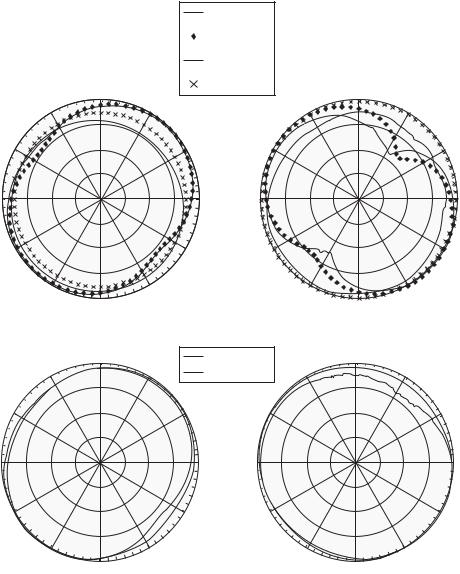
Figure 7.154 Radiation patterns of SWA (a) x–z plane (Eθ and Eϕ ), (b) y–z plane (Eθ and Eϕ ), x–z plane (|E|) and (d) y–z plane (|E|) ([75], copyright C 2009 IEEE).

patterns are illustrated in Figure 7.154, in which (a) and (b) show Eθ and Eϕ patterns on the x–z plane and y–z plane, respectively, and (c) and (d) show |E| patterns on x–z plane and y–z plane, respectively. They show almost isotropic patterns due to combined radiation from four arms in three directions which distribute energy in all directions and radiation of both horizontal and vertical polarizations for most directions.

7.2 Design and practice of ESA	187

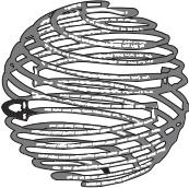
Figure 7.155 Multi-turn folded spherical helix dipole antenna ([76], copyright C 2010 IEEE).

7.2.2.2.3.4 Spherical magnetic (TE mode) dipoles

Magnetic (TE mode) dipoles can be designed to have complementary structure of electric (TM mode) dipoles. A similar folded-slot spherical helix that exhibits a magnetic dipole mode is developed by following the basic design concepts used with the folded spherical helix electric dipole [76]. The developed antenna has low VSWR, high radiation efﬁciency, and a low Q at a small value of ka. Impedance, radiation patterns, and Q properties are discussed.

Before describing the magnetic spherical helix, the electric spherical helix is introduced. As an example, a multi-turn folded spherical helix dipole is considered and the conﬁguration is shown in Figure 7.155, which depicts a single, center-fed conductor, wound around the spherical structure. The outer radius of the sphere is about 4.22 cm and the conductor diameter is 2.6 mm. Self-resonance is achieved by adjusting the total length of the conductor, and impedance matching is done by increasing the number of conductors uniformly around the surface of the imaginary sphere and connecting them at the top and bottom of the sphere. With four folded arms shown in Figure 7.155, self-resonance is achieved at 300.7 MHz, where ka = 0.266, at which the resistance is equal to 49.7 that can match to the load of 50 , radiation efﬁciency is 97%, and a Q is 84.2. This Q value is about 1.53 times the lower bound of 55.2, consistent with the limit derived by Thal [77]. Radiation pattern is given in Figure 7.156, which indicates a dominant electric dipole or TM mode (Eθ ) pattern, having omnidirectional pattern in the horizontal plane.

Here a thin wall, hollow copper sphere having an outer radius of 4.3 cm is considered and a slot is inscribed within the sphere in a shape similar to the conductors of the folded spherical helix so as to form the complementary structure. Figure 7.157 illustrates a two-arm (double slot) version of the folded slotted spherical helix. The antenna is fed horizontally at the slot located on the x–y (vertical) plane as shown in the ﬁgure. Similar to the electrical dipole version, the resonance frequency can be adjusted by increasing or decreasing the slot length. Radiation resistance can be increased by increasing the number of slots uniformly around the sphere. The two-arm version is self-resonant at a frequency of 294.86 MHz, but the radiation resistance is less than 1 . Q is 503. With increase

188	Design and practice of small antennas I

30	010	30
30	dB	30
	0
60	–10	60
	–10
	–20
90		90
120		120
150		150
	180

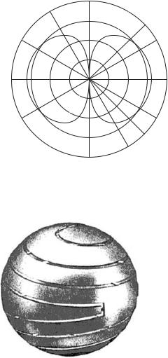
Figure 7.156 θ -sweep radiation pattern of the four-arm folded spherical helix (dominant polarization is Eθ ) ([76], copyright C 2010 IEEE).

Figure 7.157 Two-arm folded spherical helix dipole ([76], copyright C 2010 IEEE).

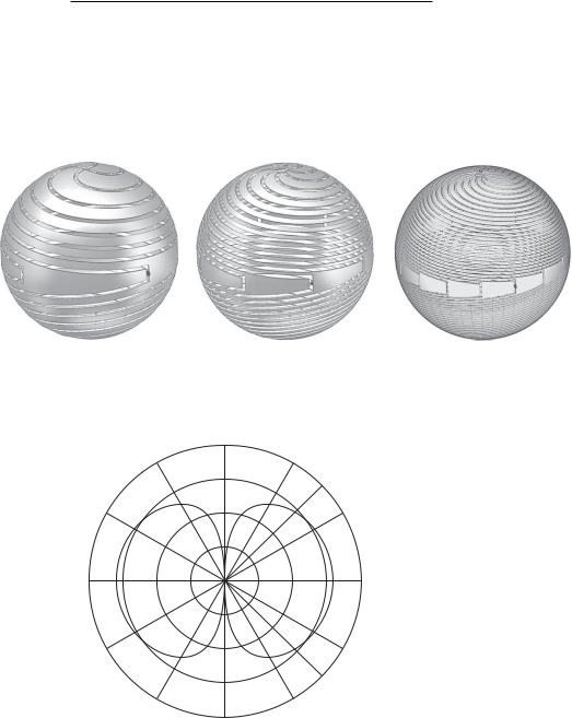
in the number of arms, radiation resistance can be increased as shown in Table 7.19; however, with 16 slots self-resonance can be achieved. The slots are connected at the top and bottom of the sphere. The 4, 8, and 16-arm versions of the antenna are illustrated in Figure 7.158(a), (b), and (c), respectively. The performances are provided in Table 7.19, where the 16-arm version shows Q of 148.5, that is about three times the lower bound. Radiation pattern of the 16-arm version is shown in Figure 7.159, which indicates a dominant magnetic dipole or TE mode (Eϕ ) pattern, having omnidirectional pattern in the vertical plane.

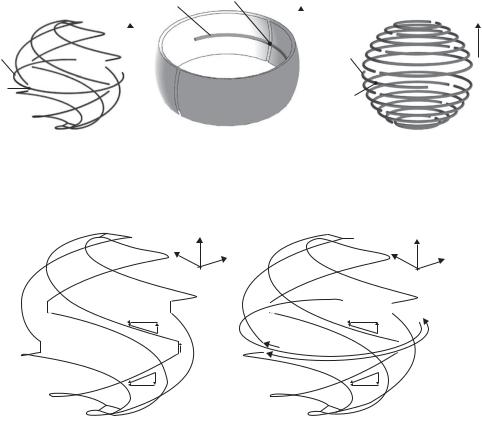
Three other modiﬁed spherical magnetic dipoles are developed [78]. Antenna conﬁgurations are illustrated in Figure 7.160, where (a) multi-arm spherical helix (MSH),

7.2 Design and practice of ESA	189

Table 7.19 Comparison of performances for the 2, 4, 8, and 16-arm folded slot spherical antennas ([76], copyright C 2009 IEEE)

	Frequency
No. Arms	(MHz)	ka	R( )	Q	VSWR

2	294.9	0.266	0.62	502.7	81.2
4	274	0.245	2.17	327.1	23
8	309.1	0.279	Not Resonant	169.6	2.33
8	310.4	0.28	15.1	173.8	3.31
16	306.4	0.276	Not Resonant	148.5	1.22

(a)

(b)

(c)

Figure 7.158 (a) Four-arm folded spherical helix dipole, (b) eight-arm folded spherical helix dipole, and (c) 16-arm folded spherical helix dipole, ([76], copyright C 2010 IEEE).

30	010	30
30	dB	30
	0
60	–10	60
	–10
	–20
90		90
120		120
150		150
	180

Figure 7.159 θ -sweep radiation pattern of 16-arm folded spherical helix dipole (dominant polarization is Eϕ ) ([76], copyright C 2010 IEEE).

190	Design and practice of small antennas I

	Excitation	Feed point
	dipole	Z
Z			Z


Excitation			Excitation

dipole			dipole

Feed point

(a)

(b)

(c)

Figure 7.160 Geometry of spherical magnetic dipole (TE10 mode) antenna: (a) multi-arm spherical helix (MSH) antenna, (b) spherical split-ring resonator (S-SRR) antenna and (c) spherical split ring (SRR) antenna, ([78], copyright C 2010 IEEE).

	Y	Z			Z
	Y	X		Y	X
		X			X
Iϕ				Iϕ
	Iθ		V	Iθ
I	V		V	I
	V
I			α	I
	Iθ			Iθ
Iϕ				Iϕ
(a)			(b)

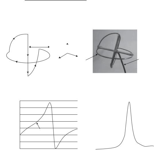
Figure 7.161 Multi-arm spherical helix (MSH) antenna: (a) TM10 (electric mode) and (b) TE10 (magnetic mode) ([78], copyright C 2010 IEEE).

(b) spherical split ring resonator (S-SRR) antenna, and (c) spherical split ring (SSR) antenna are shown.

The TE10 MSH is a modiﬁcation of a spherical helix developed by Best [72]. In the TM10 MSH antenna, the top and bottom of the arms are disconnected and a curved dipole is placed at the quarter of the antenna sphere as shown in Figure 7.161(a), where in (b) a TE10 spherical mode is also shown as a reference. The antenna is fed at the midpoint of the driven dipole by applying driving voltage horizontally so as to cancel the far-ﬁeld contribution from the θ -component produced by the electric current (Iθ ), resulting in only ﬁelds of the desired TE10 spherical mode remaining. The antenna is tuned to the resonance by changing the number of turns (Nturns) in the arm for given frequency f0 and number of arms (Narms) as is shown in Figure 7.162, where input impedance at f0 = 300 MHz is plotted for antennas of Narms = 2, 4, 6, and 8. All antennas have radius of 40 mm, and the wire radius is set to 0.5mm. The antenna occupies a spherical volume

7.2 Design and practice of ESA	191

Narms	Nturns	α,◦	Q	QLB	Q /QLB	TE10,dB	TM11,dB	TM20,dB	QLBHO	Q/QLBHO
2	2.39	163	249.6	64.6	3.87	−0.047	−22.4	−23.0	91.1	2.74
4	2.24	143	218.5	64.6	3.39	−0.030	−27.2	−23.0	90.6	24.1
6	2.19	140	210.7	64.6	3.27	−0.027	−29.5	−23.0	90.0	2.34
8	2.17	140	207.0	64.6	3.21	−0.026	−30.4	−23.0	90.0	2.30

Input impedance (kΩ)

5	Resistance
	Resistance		2 arms
4	Reactance		2 arms
4	Reactance	6 arms	4 arms
		6 arms
3	8 arms
2

1
0
−1
−2
−3
2.1	2.15	2.2	2.25	2.3	2.35	2.4	2.45	2.5

Number of turns

Figure 7.162 Input impedance of the TE10 MSH antenna as a function of number of turns in each arm ([78], copyright C 2010 IEEE).

of radius a = 40.5 mm, which corresponds to ka = 0.254 at 300 MHz. Table 7.20 summarizes the resonance state characteristics of the TE10 MSH antenna for different numbers of arms. Here QLB is the lower bound Q and QHOLB is QLB in the presence of higher modes.

The spherical split-ring resonator (S-SRR) antenna is composed of a spherical splitring resonator and a curved driven dipole arranged so as to produce mostly ϕ-directed electric surface currents, thus the desired TE10 mode. Since the antenna has symmetrical structure, it can be placed on the ground plane as Figure 7.163 illustrates. The S-SRR can be made electrically small, as the large area of the two spherical surfaces overlapped. The geometrical parameters are; r0 = a = 21 mm, t = 0.8 mm, g = 1 mm, rmnp = 18 mm, and the radius of the monopole = 0.5 mm. To achieve lower Q, the S-SRR should cover the whole sphere (β = π ); however, this results in blocking the magnetic ﬂux over the antenna cross section and thus diminishes the electric current on the antenna surface. Therefore there is an optimum coverage to yield a minimum Q. It was found the angle β = 73◦ is the optimum to obtain smallest Q/QLB. The resonance frequency depends also on the coverage and it becomes lowest when β = 64◦, which differs from the optimal β for the smallest Q/QLB, although the difference

192	Design and practice of small antennas I

t
rmnp
r0
Y
α	X
β

Z	Feed point

0.5 g

Figure 7.163 Spherical split-ring resonator (S-SRR) antenna on a ground plane ([78], copyrightC 2010 IEEE).

2γ

Feed point	0.5 g	x

Figure 7.164 Spherical split ring (SSR) antenna on a ground plane ([78], copyright C 2010 IEEE).

in the resonance frequency is minor, being only 1.5 MHz. For β = 73◦, the resonance frequency f0 is 297.0 MHz and ka = 0.133. The input impedance can be adjusted by the length of the driven dipole, and with α = 55◦, the input resistance at the resonance R0 is 50 for the optimal β = 73◦. The lowest Q/Qlb obtained is around 3.4, which is nearly the same as that of MSH.

The spherical split ring (SSR) antenna consists of individual wire split rings distributed evenly in θ as shown in Figure 7.160(c). Every two neighbor rings are ﬂipped with respect to each other and thus, operate as a conventional SRR. Multi-element SRR is constituted by combining rings with other rings so that uniform current distribution over the spherical surface is realized and the resonance frequency is lowered. The number of the rings is chosen to be odd, so that the antenna is driven at the central split ring, the length of which is adjusted to attain the input impedance to match the feed line. Since the SSR has symmetrical structure, it can be made in half and mounted on the ground plane as shown in Figure 7.164. The resonance frequency is changed by the number of split rings Nsr and is determined by using the following expression

Nsr = 2int(90◦/γ ) − 1

(7.68)

<<< < Предыдущая 29 30 31 32 33 34 35 36 37 38 39 4041 / 8941 42 43 44 45 46 47 48 49 50 51 52 53 > Следующая >>>

Соседние файлы в папке OC

#
15.12.20186.46 Mб217Broadband microstrip antennas.pdf
#
15.12.20189.36 Mб114fujimoto_kyohei_morishita_hisashi_modern_small_antennas.pdf