Figure 6.30 Current distribution on a short dipole; (a) triangular shape and (b) uniform (ideal case).

Figure 6.31 Capacitance plate loaded on the top of a short dipole.

Figure 6.32 A capacitance loaded transmission line.

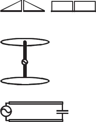
to obtain uniform current distribution on a short dipole is to place a capacitance plate loading on its top as shown in Figure 6.31 [38]. By this means, the antenna gain can be the highest that is possible with that length of the dipole antenna. The longer the linear part of the antenna becomes, the nearer the current distribution approaches to uniform, as the distribution is gradually smoothed from the triangle. By loading a capacitor at the end terminal, the current distribution on the transmission line may be made nearly uniform (Figure 6.32).

6.2.4Increase of radiation modes

Increasing radiation modes is another important method to create an ESA. Hansen discussed in [30] that antenna Q will be reduced by 1/2 with simultaneous excitation of TE and TM modes. Reduction of antenna Q implies increase in the bandwidth. If this can be achieved in an antenna with a given size, it corresponds to creating an ESA. Practical methods to increase radiation modes are composing an antenna with complementary structure, or conjugate structure, combining different types of antenna, and so forth. These will be described in the following section.

Figure 6.33 A demonstration of the principle of self-complementary concept combining two (E and H) mode structure [39].

Monopole

Slot

Figure 6.34 An example of self-complementary antenna; composed with a monopole and a complementary slot on the ground plane [40].

6.2.4.1Use of self-complementary structure

Self-complementary structure is constructed by combining two-mode (E and H) structures [39], as Figure 6.33 illustrates. An example is a monopole combined with a self-complementary shape of a slot on the ground plane as shown in Figure 6.34 [40, 41]. A self-complementary antenna has inherently frequency independent properties, as the impedance Z0 of a complementary antenna is constant over infinite frequency range as shown by Mushiake in [40] with

where Z1 is the impedance of an E-mode antenna, Z2 is that of a complementary H-mode antenna, and Z0 is the intrinsic impedance of the medium.

The perfect frequency independent performance can be achieved only when the size of the ground plane is infinite. With a finite ground plane, the property of frequency independence is limited to some extent, and the frequency bandwidth is no longer infinite, although the bandwidth obtained will be still appreciably wide.

Some examples of planar self-complementary antennas are shown in Figure 6.35 [39].

Figure 6.35 Examples of planar self-complementary structures [39].

6.2.4.2Use of conjugate structure

An antenna composed of conjugate components consisting of a capacitive element and its conjugate inductive element so that the reactive component in the antenna structure can be compensated, resulting in self-resonance, can be designed to have appreciably wide bandwidth, although the size is fairly small. This is also a useful method to produce an ESA. Combination of an electric source with a magnetic source may become a pair to compensate the reactive component in the antenna structure; thus self-resonance is attained.

6.2.4.3Compose with different types of antennas

It has been shown in the previous sections that radiation modes of an antenna can be increased by increasing radiation sources, realized by combining different types of antennas, which contribute to producing different radiation modes. In addition to previously described methods such as complementary and conjugate structures, other examples are introduced below.

An example is an ESA composed with a small loop and a ground plane, on which the receiver circuit is mounted [42]. The antenna is designed based on the concept for producing ESA; increasing radiation modes, and accomplishing self-resonance. Figure 6.36 illustrates an antenna system as an example, where a loop antenna is located inside a small unit and fed with a coaxial cable. The antenna system is expressed as a combination of a loop element and the ground plane (printed circuit board) as Figure 6.37(a) shows. At the feed terminals of this antenna system, the current I0 flows, that can be divided

Figure 6.36 An example of a composite antenna system composed of a loop and a dipole [41b].

Figure 6.37 Equivalent expression of the antenna system shown in Figure 6.36; (a) the antenna system, (b) the loop and (c) an equivalent dipole composed with the loop and the ground [41b].

into two modes; one part is the unbalanced current Iu and another is the current Ib. These two modes are originated from feeding the connection of the loop with an unbalanced cable. The balanced current Ib flows into the balanced terminals of the loop as shown in Figure 6.37(b), while the unbalanced current Iu, flows into both the ground plane and the loop element as Figure 6.37(c) shows. Because of the unbalanced current flow on the loop element, the loop element can be assumed to be an equivalent flat plate that yields a virtual planar dipole along with the ground plane as Figure 6.38 depicts.

This antenna was previously used in a VHF pager and brought several significant outcomes that were: (1) about a 3 dB increase in the receiver sensitivity when the pager was put in the operator’s pocket due to the image effect of the loop, and (2) a change in the receiving pattern (sensitivity) to almost non-directional as a result of combination of a figure-eight pattern of the loop and another out-of-phase figure-eight pattern of the equivalent dipole. This antenna system simply appears to be only a small loop, but actually works with enhanced performance as a consequence of two-mode combination of a loop and a virtual dipole.