

138 |
Design and practice of small antennas I |
|||||||||||
|
|
|
|
|
|
|
|
|
|
|
|
|
|
|
|
|
|
|
|
|
|
|
|
|
|
|
|
|
|
|
|
|
|
|
|
|
|
|
|
|
|
|
|
|
|
|
|
|
|
|
|
|
|
|
|
|
|
|
|
|
|
|
|
|
|
|
|
|
|
|
|
|
|
|
|
|
|
|
|
|
|
|
|
|
|
|
|
|
|
|
|
|
|
|
|
|
|
|
|
|
|
|
|
|
|
|
|
|
|
|
|
|
|
|
|
|
|
|
|
|
|
|
|
|
|
|
|
|
|
|
(a) |
(b) |
|
|
(c) |
|||||||
|
|
|
|
|
|
|
|
|
|
|
|
|
|
|
|
|
|
|
|
|
|
|
|
|
|
|
|
|
|
|
|
|
|
|
|
|
|
|
|
|
|
|
|
|
|
|
|
|
|
|
|
|
|
|
|
|
|
|
|
|
|
|
|
|
|
|
|
|
|
|
|
|
|
|
|
|
|
|
|
|
|
|
|
|
|
|
|
|
|
|
|
|
|
|
|
|
|
|
|
|
|
|
|
(d) |
(e) |
(f) |
|
|
|
|
|
|
|
|
|
(g) |
(h) |
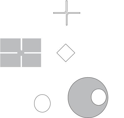
Figure 7.78 Variations of slots/slits on the rectangular patch: (a) cross slot, (b) a pair of bent slots,
(c) a group of four bent slots, (d) four slits on the center of each side, (e) a square slot, (f) four rectangular slots, (g) a circular slot, and (h) an offset circular slot [29].
the size. For that purpose, slots and slits are combined to enhance the performance and achieve downsizing as well. The FSAs will be described in the next chapter.
7.2.2Full use of volume/space
The concept of filling volume/space by an antenna element is based on Wheeler’s work showing that antennas fully utilizing the volume that circumscribes the maximum size of an antenna, will provide the lowest Q as compared with other geometries within the same volume. He examined the antenna Q in relation to the antenna size by taking a cylindrical shape of capacitor and inductor representing a C-type and an L-type dipole
7.2 Design and practice of ESA |
139 |
|
|
2a
A = a2
(a) |
b |
(b) |
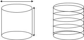
Figure 7.79 (a) Small C-type antenna and (b) L-type antenna occupying the same volume ([30], copyright C 1947 IEEE).
antenna, respectively, as is depicted in Figure 7.79, and he showed that the Q is inversely proportional to the volume of the antenna [30]. In his analysis, Wheeler used circuit parameters, capacitor C, inductance L, and radiation resistance Rrad or conductance Grad of these antennas, and derived Q. The C and L became:
C = ε0kC A/b |
(7.48) |
L = μ0π 2 A/ kL b |
(7.49) |
where kC and kL, respectively, are the shape factor of the C-type and the L-type antenna, A denotes the cross section area, and b is the height, as Figure 7.79 shows.
Radiation resistance Rrad and conductance Grad, respectively, are derived as
RCrad = 20(kb)2, and GCrad = (k2kC A)/(6π Z0) |
(7.50) |
for the C-type antenna, and
RLrad = 20(nk2 A)2, and GLrad = (kkL A)2/(6π n2 Z0) |
(7.51) |
for the L-type antenna.
Here k is the wave number (2π /λ), n is number of turns of the coil, and Z0 is the free space impedance. Then by using Eqs. (7.48–7.50), QC of the C-type antenna and QL of the L-type antenna, respectively, are derived as
QC = ωC/GC = 6π k3/(kC Ab) = 9VRS /2Veff |
(7.52) |
and |
|
QL = ωL/RL = 6π k3/(kL Ab) = 9VRS /2Veff |
(7.53) |
where VRS denotes the volume of a sphere having radius λ/2π (the radian sphere), and Veff is the effective volume, which is defined by
Veff = σ Vphy . |
(7.54) |
Here σ = kC, kL and Vphy is the physical volume of the antenna.
Equations (7.52) and (7.53) indicate that Q is inversely proportional to Veff, thus Vphy, as Vphy is proportional to Veff, and that by constituting an antenna in a sphere, which
140 |
Design and practice of small antennas I |
|
|
μr
μ0 |
2a |
|
n turns
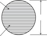
Figure 7.80 Wheeler’s spherical coil ([31], copyright C 1958 IEEE).
encloses its minimum, so as to occupy the entire volume of the sphere, the lowest Q will be obtained.
Wheeler examined what type of small antenna can most effectively utilize the volume or has the highest volume and lowest Q. He took up a constant pitch spherical coil of n turns with magnetic core as shown in Figure 7.80 [31], where the excitation voltage is across the poles of the coil, and he calculated the circuit parameters, from which Q can be found as
Q = (1 + 2/μr )/(ka)3 = VRS /(σ Vphy ). |
(7.55) |
Where μr is the relative permeability of material filled in the sphere, and a is the radius of the sphere. The lowest Qmin is obtained when μr is infinite; that is,
Qmin = 1/(ka)3. |
(7.56) |
It should be noted that this is a case for an antenna radiating only either TE10 or TM10 mode. When both TE10 and TM10 are radiated, Qmin becomes
Qmin = 1/2(ka)3. |
(7.57) |
Chu worked on a similar problem. There is a well-known bound for Q that is often referred to as the Chu limit; the theoretical minimum Q relates to the spherical volume, which embraces the maximum dimensions of the antenna. Here assuming a hypothetical sphere having radius a, the Chu limit [32] prescribes that the lower bound of Q is a function of ka (k = 2π /λ), the dimensional parameter of the sphere, and is given by
Q = (ka3)−1 + (ka)−1. |
(7.58) |
To obtain a Q of the closest lower bound of Eq. (7.58), the antenna must effectively utilize the total sphere volume defined by the dimensional parameter ka. In case of a thin linear dipole having length l and diameter d, a hypothetical sphere which circumscribes the dipole should have the radius l/2, and hence the dipole occupies only a small part of the volume of the sphere, implying very inefficient use of the volume of the sphere. Meanwhile, in case of a spherical dipole, which occupies the outermost regions of the sphere of radius l/2, the volume of the sphere is utilized very efficiently. The lowest Q may be closely approached by this sort of spherical dipole.
The concept of filling volume can be applied to the two-dimensional case; that is, when a space is occupied fully with thin metallic conductors a lower obtainable Q
7.2 Design and practice of ESA |
141 |
|
|
(a)
|
|
|
|
|
|
|
|
|
|
|
|
|
|
|
|
|
|
|
|
|
|
|
|
|
|
|
|
|
|
|
|
|
|
|
|
|
|
|
|
|
|
|
|
|
|
|
|
|
|
|
|
|
|
|
|
|
|
|
|
|
|
|
|
|
|
|
|
|
|
|
|
|
|
|
|
|
|
|
|
|
|
|
|
|
|
|
|
|
|
n = 1 |
|
|
|
n = 2 |
|
|
|
|
|
|
|
|
|
n |
|
= 3 |
|
|
|
|
|
|
|||||||
(b)
n = 1 |
n = 2 |
n = 3 |
n = 4 |
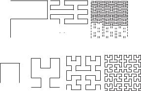
Figure 7.81 (a) Peano curve; order one through three and (b) Hilbert curve; order one through four [33].
can be achieved within a limited space. For this purpose, the concept of space-filling curves, which are generally a continuous mapping of the normalized interval onto the normalized square, is used. The space-filling curve was first proposed by G. Peano in 1890 [33], and now it is called the Peano curve. D. Hilbert introduced his version of space-filling curve in 1891 [33], now called the Hilbert curve. These curves are composed through iterative generating procedures, by which contours (patterns) with infinitely complicated structure to fill a space are produced. The pattern is formed by infinitely repeating combinations of scaling and rotating an initial pattern. It is expressed in terms of the iteration numbers and the space is gradually filled as the iteration number approaches infinity. Figure 7.81(a) illustrates Peano curves of orders n = 1 through 3 and (b) shows Hilbert curves of orders n = 1 through 4.
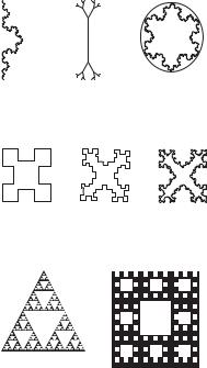
In addition to these two curves, fractal patterns are also known as a class of spacefilling curve, and have been used for lowering resonance frequency and thus small sizing of antennas. Fractal stands for “Fractional Dimension,” and incorporates the meaning of “fragmented” or “broken.” The term fractal has been applied to a species of cumulus clouds or stratus clouds with ragged, shred appearance. The fractal patterns are produced by similar iteration procedures, starting from a “generator,” which replaces an “initiator,” the initial geometry, and repeats this iteration process infinitely. Representative Fractals include Koch [34a], Minkowsky [34b], and Sierpinsky [34c], respectively, as shown in Figures 7.82, 7.83, and 7.84. In the case of a Koch Fractal, the initiator is a line, and onethird of the line is replaced by the generator, which is an equilateral triangle, at its center, and this procedure is repeated an infinite number of times to create a geometry that has intricate patterns on an ever-shrinking scale.
These fractal structures are expressed in terms of iteration number. In addition, as the iteration order of the pattern increases, the length of the element increases, while the footprint area is maintained the same. By this means, the resonance frequency is lowered without increasing the space, and hence it can be used for creating small antennas. Furthermore, when it is used for an antenna, it offers another advantage that input impedance can be increased as the length of the fractal pattern element increases,
142 |
Design and practice of small antennas I |
|
|
Figure 7.82 Koch fractal models ([34a], copyright C 2000 IEEE).
Figure 7.83 Minkowsky fractal models ([34b], copyright C 2002 IEEE).
Figure 7.84 Sierpinsky fractal models ([34c], copyright C 2003 IEEE).
whereas an ordinary small antenna suffers having very small input impedance that hinders good matching.
Features of space-filling curves, including fractal structures, when applied to antennas, result in not only lowering the resonance frequency, and increasing antenna impedance, but also in increasing the surface impedance as a result of lengthened space-filling elements within the limited space, that will produce a high impedance surface (HIS). The HIS can offer various salient antenna performances and novel antenna structure, and can decrease mutual coupling between antenna elements. Furthermore, enhancement of the antenna performance is attained by utilizing positive image effects, and a decrease of coupling between antenna elements allows close location of several antenna elements on a limited space, that will bring an increase in the transmission data-rate when it is applied to the MIMO system. Suppression of surface current contributes to decreasing undesired radiation; for instance, resulting in increase of the front-to-back ratio due to the reduction of backward radiation.
Spiral patterns are considered as a class of space-filling pattern as they occupy an area of given size without much vacancy and contribute to making bandwidth wide. This does not necessarily imply small-sizing of an antenna in terms of an entire frequency range, but at the lower resonance frequencies the antenna should be recognized as small-sized in terms of the operating wavelength. Then, spiral antennas should be partially classified into Functionally Small Antenna and partially into Electrically Small Antenna.