

7.2 Design and practice of ESA |
103 |
|
|
|
1000 |
|
|
|
|
|
|
|
|
|
|
|
|
|
|
|
|
|
|
|
Ω) |
|
|
|
|
|
|
|
|
|
|
|
|
|
w |
|
|
|
|
|
|
|
|
|
|
|
|
|
|
|
|
|
|
|
|
|
||||||
( |
|
|
|
|
|
|
|
|
|
|
|
|
|
|
|
|
|
|
|
|
c |
|
|
|
|
|
|
|
|
|
|
|
|
|
εr |
|
|
|
|
|
t |
Z |
|
|
|
|
|
|
|
|
|
|
|
|
|
|
|
|
|
|
||
impedance |
100 |
|
|
|
|
|
|
|
|
|
|
|
Two-strip |
|
||||||
|
|
|
|
|
|
|
|
|
|
|
|
|
||||||||
Characteristic |
|
|
|
|
2a |
|
|
|
|
|
|
|
|
|
|
|
|
|
|
|
|
|
|
|
|
|
|
|
|
|
|
|
|
|
|
|
|||||
10 |
|
|
|
|
|
t |
|
|
εr = 1 |
|
||||||||||
|
|
|
|
|
|
|
|
|
||||||||||||
|
|
|
|
|
|
|
|
|
||||||||||||
|
|
|
|
|
|
|
|
|
||||||||||||
|
|
|
|
|
|
|
|
|
|
|||||||||||
|
|
|
|
|
|
|
|
|
|
|
|
|
||||||||
|
|
Two-wire |
|
|
2.6 |
|
|
|
|
|
||||||||||
|
|
|
|
|
|
|
|
|
|
|
|
|
||||||||
|
1 |
0.1 |
|
|
|
1 |
|
10 |
|
|
|
|
100 |
|||||||
|
0.01 |
|
|
|
|
|
|
|
|
|||||||||||
2a/t for two-wire w/t for two-strip
Figure 7.18 Relationship between Zc and wire radius a in terms of t (from [10]).
Figure 7.9, Z0 is expressed as shown in Figure 7.18. These are useful for designing an antenna consisting of two parallel strip-type meander lines.
A practical model having h = 0.11λ (144.4 mm), d = 0.057λ (74.8 mm), and N (number of segments) = 6, is considered. In this case, f0 is set to 228 MHz, Sm = 1.5, and the thickness of the substrate (Teflon, ε = 2.6) is 0.0006λ (0.8 mm). From Figure 7.14 and Figure 7.15, um is 1.1 and RBW is 0.013. When the elements 1 and 2 are connected at the end to form the folded structure, L/λ becomes 0.75, and Z0 is found to be 9.58 . From these, w/t is 18, and thus w becomes 0.011λ (14.4 mm), as t = 0.8 mm. RBW is obtained to be about 7.2%. Measured impedance (200 MHz step between 200 and 260 MHz) is shown in Figure 7.19, where a square ground plane of 0.76 λ (1 m) is used. Radiation efficiency obtained was about 90% to 95%. Sm in terms of frequency f is shown in Figure 7.20.
A tapered folded-type MLA is described in [9a], including folded type with a plate top-loaded MLA.
7.2.1.1.1.1.4 Meander line antenna mounted on a rectangular conducting box
When an MLA is mounted on a rectangular conducting box [12], as can be often seen in practical applications (Figure 7.21), the resonance frequency fr varies with the distance S of the antenna element from the surface of the substrate on which the antenna is printed. R and fr with respect to S are given in Figure 7.22. Figure 7.23 illustrates impedance loci on the Smith chart. The locus A is for the MLA mounted on the rectangular box, while the locus B is for the MLA placed on a circular ground plane with a diameter of 1 m. In both cases the impedance loci encircle near the center of the Smith chart, providing evidence of wideband characteristics. The frequency range used in the measurement is between 800 MHz and 900 MHz.

0
+j
|
5 |
1 |
. |
≤ |
|
R |
|
∞
W
S
V
−j
Figure 7.19 Measured impedance ([10], copyright C 1999 IEICE).
u
VSWR
−3 −2 −1 0 |
1 |
2 |
3 |
3 |
|
|
|
2.5
2
1.5
1 |
|
|
|
|
210 |
220 |
230 |
240 |
250 |
Frequency (MHz)
 CalculatedMeasured )
Figure 7.20 VSWR Sm versus frequency f ([10], copyright C 1999 IEICE). |
||
|
Feed |
Ground |
|
z |
|
|
|
y |
|
|
S |
|
|
x |
|
h |
t = 0.2 |
120 |
p |
d = 24.9 |
|
p = 8 |
|
|
|
|
|
d |
h = 32 |
|
t |
[mm] |
|
|
28 |
|
40 |
|
Figure 7.21 An MLA mounted on a conducting box ([12], copyright C 1999 IEICE).
7.2 Design and practice of ESA |
105 |
|
|
Frequency (MHz)
750 |
|
|
700 |
fr |
|
R |
||
|
||
650 |
|
|
600 |
S |
|
|
||
550 |
|
2 6 10 14 18
S (mm)
15 |
|
|
10 |
(Ω) |
|
Resistance |
||
5 |
||
|
||
0 |
|
Figure 7.22 Resonance frequency fr and radiation resistance R with respect to distance S ([12], copyright C 1999 IEICE).
A
S = 7mm
800 MHz
VSWR≤− 2 |
B |
|
S = 10mm |
||
|
Figure 7.23 Impedance loci of MLAs: a two-wire type mounted on a rectangular conducting plate and a one-wire type mounted on a circular conducting plane ([12], copyright C 2004 IEICE).
7.2.1.1.1.1.5 Small meander line antennas of less than 0.1 wavelength [13]
Small meander line dipole-type antennas having their lengths smaller than 0.1λ have been extensively studied theoretically and experimentally, and the design parameters have been provided [13]. The basic antenna structure is shown in Figure 7.24, where antenna dimensional parameters are given. The antenna performance was calculated by using an EM simulator IE3D and the operating frequency is taken to be 700 MHz. Since the wire width d of the element is considered one of the significant parameters in designing the antenna, when the antenna length L is first set to a desired value, the number N of meandering turns is determined in conjunction with the width d. In this case, d is the maximum value dmax that is determined by the desired length L. Figure 7.25 shows dmax in relation to the number N for different L (from 0.025 λ to 0.1 λ) of the antenna length where the separation s of wire elements is 0.1 mm. This type of antenna can easily be set in self-resonance condition, as the wire length La of the antenna can be made long enough to be nearly a quarter wavelength by selecting the number N and the antenna width W appropriately. Relationships between W/λ and L/λ in the resonance condition are given in Figure 7.26, where N is used as the parameter. In the figure, two cases when d is 0.3mm (2.3 × 10 −4 λ) and 0.1mm (7.0 × 10⁻⁴ λ), respectively, are
106 |
Design and practice of small antennas I |
|
|
d |
s |
|
Lf |
|
W |
L
Figure 7.24 MLA model with the length less than 0.1λ ([13], copyright C 2004 IEICE).
Conductor width dmax (mm)
1.5 |
|
|
|
|
|
|
|
|
|
|
|
|
d |
|
|
|
|
|
|
|
|
|
|
|
|
|
|
|
|
|
|
|
|
|
|
|
s = 0.1 mm |
|
|||
1 |
|
|
|
|
|
|
|
|
|
|
|
|
|
|
|
|
|
|
|
|
|
|
|
|
|
|
|
|
|
|
|
|
|
|
|
|
|
|
|
|
|
|
|
|
|
|
|
|
|
|
|
|
|
|
|
|
|
|
|
|
|
|
|
|
|
|
|
|
|
|
|
|
|
|
|
|
|
|
|
|
|
|
|
|
|
|
|
|
|
|
|
|
|
|
L = 0.1λ |
|
|
|
||||||
|
|
|
|
|
|
|
|
|
|
|
|
|
||||||||
|
|
|
|
|
|
|
|
|
|
|
|
|
|
|
||||||
0.5 |
|
|
|
|
|
|
|
|
|
L = 0.075λ |
|
|
|
|||||||
|
|
|
|
|
|
|
|
|
|
|
|
|||||||||
|
|
|
|
|
|
|
|
|
L = 0.05λ |
|
|
|
||||||||
|
|
|
|
|
|
|
|
|
|
|
||||||||||
|
|
|
|
|
|
|
|
|
|
|
|
|
||||||||
0 |
|
|
|
|
|
|
|
|
|
L = 0.025λ |
|
|
|
|||||||
|
|
|
|
|
|
|
|
|
|
|
|
|||||||||
|
|
|
|
|
|
|
|
|
|
|
|
|||||||||
|
|
|
|
|
|
|
|
|
|
|
|
|
|
|
|
|
|
|
|
|
|
|
22 |
38 |
46 |
|
62 |
||||||||||||||
10 |
|
|||||||||||||||||||
N
Figure 7.25 Antenna width dmax with respect to the segment number N ([13], copyright C 2004 IEICE).
|
0.1 |
|
/λ) |
0.08 |
|
(W |
||
|
||
width |
0.06 |
|
Antenna |
0.04 |
|
|
||
|
0.02 |
|
|
0.025 |
d = 0.3 mm |
, |
N = 10 |
d = 0.1 mm |
, |
N = 22 |
|
, |
N = 38 |
|
|
|
|
|
|
|
|
|
|
|
|
|
|
|
|
|
|
|
|
|
0.05 |
0.075 |
0.1 |
||||
Antenna length (L/λ)
Figure 7.26 Antenna width w/λ with respect to the wire length L/λ ([13], copyright C 2004 IEICE).
7.2 Design and practice of ESA |
107 |
|
|
d = 0.3 mm |
, |
N = 38 |
d = 0.1 mm |
, |
N = 22 |
) |
, |
N = 10 |
Wire length (La/λ |
|
|
Antenna length (L/λ)
Figure 7.27 Wire length La versus antenna length L at resonance state ([13], copyright C 2004 IEICE).
|
25 |
|
: N = 10 |
|
|
|
|
|
|
|
|
d = 0.3 mm |
|
|
|||
|
20 |
|
: N = 22 |
|
|
|||
|
|
: N = 38 |
|
|
|
|
||
L |
15 |
|
|
|
|
|
|
|
, R |
|
|
|
|
|
|
Rin |
|
in |
|
|
|
|
|
|
|
|
R |
10 |
|
|
|
|
|
RL |
|
|
|
|
|
|
|
|
||
|
|
|
|
|
|
|
|
|
|
5 |
|
|
|
|
|
|
|
|
0 |
|
|
|
|
|
|
|
|
0.025 |
0.05 |
0.075 |
0.1 |
0.125 |
0.15 |
0.175 |
0.2 |
Antenna length (L/λ)
Figure 7.28 Input resistance Rin and loss resistance Rl with respect to the antenna length L/λ ([13], copyright C 2004 IEICE).
shown. The antenna wire length La/λ in relation with L/λ at the self-resonance state is illustrated in Figure 7.27 for cases d = 0.1 and 0.3, and N = 10, 22, and 38.
Input resistance Rin and loss resistance RL of an antenna in relation to the antenna length L/λ for cases N = 10, 22, and 38, and d = 0.3 are shown in Figure 7.28. The loss resistance Rl of a conductor with the skin depth δ and the conductivity σ is given by
Rl = 1/(δσ ), |
(7.26) |
||
where δ = |
1/( f π μσ ) |
. |
(7.27) |
When the conductor has planar structure with length L, width w, and thickness t, loss resistance RL of an antenna is expressed by
√
RL = Rl L/2(w + t) = L σ f π μ/2(w + t). (7.28)
When the conductor is copper, σ is 5.8 × 10⁷ [S/m], then δ = 2.5 mm at 700 MHz.
√
Since RL increases with the antenna wire length La and f , when L becomes less than 0.1λ, it increases notably with increase in N that makes La large.
108 |
Design and practice of small antennas I |
|
|
|
0.12 |
|
/λ) |
|
|
(W |
0.08 |
|
width |
||
|
||
Antenna |
0.04 |
|
|
||
|
0 |
|
|
0.05 |
Theory |
d = 0.3 mm |
Simulation |
N = 10
N = 22
N = 38
0.1 |
0.15 |
0.2 |
Antenna length (L/λ)
Figure 7.29 Relationship between antenna length L/λ and antenna width w/λ ([13], copyrightC 2004 IEICE).
d
(a)
Lf |
L |
s |
L |
|
|
(b) |
|
W |
|
W |
W′ |
L
W
(c)
Figure 7.30 Typical structure of folded-type MLA: (a) dipole type, (b) a folded-back type, and
(c) folded-up type ([13], copyright C 2004 IEICE).
Relationships between the antenna length L/λ and the antenna width W for cases N = 10, 22, and 38 and d = 0.3 are shown in Figure 7.29.
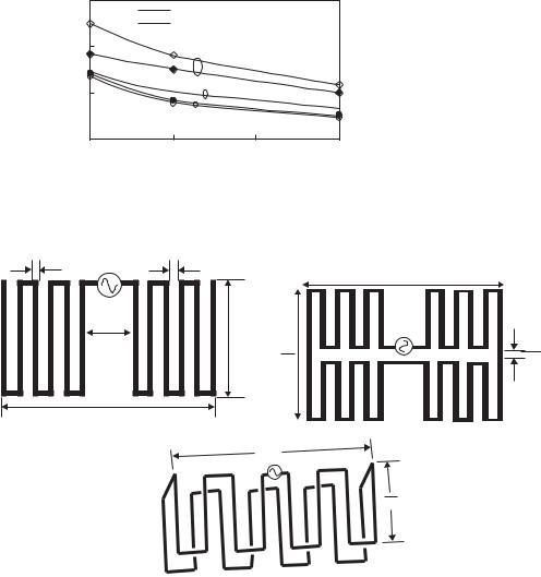
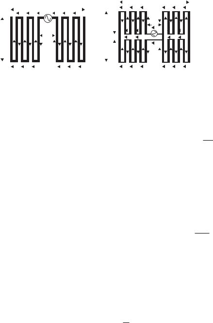
When an antenna is a folded type, increase in the antenna impedance is expected. Figure 7.30 illustrates two types of folded MLAs along with an original dipole-type MLA (hereafter called “dipole-type” MLA); (a) is a dipole-type MLA, (b) is a foldedback type MLA, and (c) is a folded-up type MLA. The current distributions on an MLA are shown in Figure 7.31, in which arrows indicate directions of the current flows. Figure 7.31(a) depicts current flows on a dipole type and (b) that on a folded type. These figures suggest that substantial radiation is produced by the currents on the horizontal
|
|
|
|
|
|
|
|
|
|
|
|
|
|
|
|
|
|
|
|
|
|
|
|
|
|
|
|
|
|
|
|
|
|
|
|
|
|
|
|
|
|
|
|
|
|
|
|
|
|
|
|
7.2 Design and practice of ESA |
109 |
|||||||||||||||||||||||||||||||||||||||||||||
|
|
|
|
|
|
|
|
|
|
|
|
|
|
|
|
|
|
|
|
|
|
|
|
|
|
|
|
|
|
|
|
|
|
|
|
|
|
|
|
|
|
|
|
|
|
|
|
|
|
|
|
|
|
|
|
|
|
|
|
|
|
|
|
|
|
|
|
|
|
|
|
|
|
|
|
|
|
|
|
|
|
|
|
|
|
|
|
|
|
|
|
|
|
|
|
|
|
|
|
|
|
|
|
|
|
|
|
|
|
|
|
|
|
|
|
|
|
|
|
|
|
|
|
|
|
|
|
|
|
|
|
|
|
|
|
|
|
|
|
|
|
|
|
|
|
|
|
|
|
|
|
|
|
|
|
|
|
|
|
|
|
|
|
|
|
|
|
|
|
|
|
|
|
|
|
|
|
|
|
|
|
|
|
||||||||||||||
|
|
|
|
|
|
|
|
|
|
|
|
|
|
|
|
|
|
|
|
|
|
|
|
|
|
|
|
|
L |
|
|
|
|
|
|
|
|
|
|
|
|
|
|
|
|
|
|
|
|
|
|
|
|
|
|
|
|
|
|
|
|
|
|
|
|
|
|
|
|
|
|
|
|
|
|
|
|
L |
|
|
|
|
|
|
||||||||||||||
|
|
|
|
|
|
|
|
|
|
|
|
|
|
|
|
|
|
|
|
|
|
|
|
|
|
|
|
|
|
|
|
|
|
|
|
|
|
|
|
|
|
|
|
|
|
|
|
|
|
|
|
|
|
|
|
|
|
|
|
|
|
|
|
|
|
|
|
|
|
|
|
|
|
|
|
|
|
|
|
|
||||||||||||||||||
|
|
|
|
|
|
|
|
|
|
|
|
|
|
|
|
|
|
|
|
|
|
|
|
|
|
|
|
|
|
|
|
|
|
|
|
|
|
|
|
|
|
|
|
|
|
|
|
|
|
|
|
|
|
|
|
|
|
|
|
|
|
|
|
|
|
|
|
|
|
|
|
|
|
|
|
|
|
|
|
|
|
|
|
|
|
|
|
|
|
|
|
|
|
|
|
|
|
|
|
|
|
|
|
|
|
|
|
|
|
|
|
|
|
|
|
|
|
|
|
|
|
|
|
|
|
|
|
|
|
|
|
|
|
|
|
|
|
|
|
|
|
|
|
|
|
|
|
|
|
|
|
|
|
|
|
|
|
|
|
|
|
|
|
|
|
|
|
|
|
|
|
|
|
|
|
|
|
|
|
|
|
|
|
|
|
|
|
|
|
|
|
|
|
|
|
|
|
(a) |
|
|
|
|
|
|
|
|
|
|
|
|
|
|
|
|
|
|
|
|
|
|
|
|
|
|
|
|
Lf |
|
|
|
|
|
|
|
|
|
|
|
|
|
|
|
|
|
(b) |
|
|
W′ |
|
|
|
|
Lf |
|
|
|
|
|
|
|||||||||||||||||||||||||||||||||||||
|
|
|
|
|
|
|
|
|
|
|
|
|
|
|
|
|
|
|
|
|
|
|
|
|
|
|
|
|
|
|
|
|
|
|
|
|
|
|
|
|
|
|
|
|
|
|
|
|
|
|
|
|
|
|
|
|
|
|
|
|
|
|
|
|
|
|
|
|
|
|
|
|
|
|
|
|
|
|
|
|||||||||||||||||||
|
|
|
|
|
|
|
|
|
|
|
|
|
|
|
|
|
|
|
|
|
|
|
|
|
|
|
|
|
|
|
|
|
|
|
|
|
|
|
|
|
|
|
|
|
|
|
|
|
|
|
|
|
|
|
|
|
|
|
|
|
|
|
|
|
|
|
|
|
|
|
|
|
|
|
|
|
|
|
|
|
|
|
|
|||||||||||||||
|
|
|
|
|
|
|
|
|
|
|
|
|
|
|
|
|
|
|
|
|
|
|
|
|
|
|
|
|
|
|
|
|
|
|
|
|
|
|
|
|
|
|
|
|
|
|
|
|
|
|
|
|
|
|
|
|
|
|
|
|
|
|
|
|
|
|
|
|
|
|
|
|
|
|
|
|
|
|
|
|
|
|
|
|
|
|
|
|
|
|
|
|
|
|
|
|
|
|
|
W |
|
|
|
|
|
|
|
|
|
|
|
|
|
|
|
|
|
|
|
|
|
|
|
|
|
|
|
|
|
|
|
|
|
|
|
|
|
|
|
|
|
|
W |
|
|
|
|
|
|
|
|
|
|
|
|
|
|
|
|
|
|
|
|
|
|
|
|
|
|
|
|
|
|
|
|
|
|
|
|
|
|
|
|
|
|
|
|
|
|||||||||
|
|
|
|
|
|
|
|
|
|
|
|
|
|
|
|
|
|
|
|
|
|
|
|
|
|
|
|
|
|
|
|
|
|
|
|
|
|
|
|
|
|
|
|
|
|
|
|
|
|
|
|
|
|
|
|
|
|
|
|
|
|
|
|
|
|
|
|
|
|
|
|
|
|
|
|
|
|
|
|
|
|
|
|
|
|
|
|
|
|
|
|
|
|
|
|
|
|
|
|
|
|
|
|
|
|
|
|
|
|
|
|
|
|
|
|
|
|
|
|
|
|
|
|
|
|
|
|
|
|
|
|
|
|
|
|
|
|
|
|
|
|
|
|
|
|
|
|
|
|
|
|
|
|
|
|
|
|
|
|
|
|
|
|
|
|
|
|
|
|
|
|
|
|
|
|
|
|
|
|
|
|
|
|
|
|
|
|
|
|
|
|
|
|
|
|
|
|
|
|
|
|
|
|
|
|
|
|
|
|
|
|
|
|
|
|
|
|
|
|
|
|
|
|
|
|
|
|
|
|
|
|
|
|
|
|
|
|
|
|
|
|
|
|
|
|
|
|
|
|
|
|
|
|
|
|
|
|
|
|
|
|
|
|
|
|
|
|
|
|
|
|
|
|
|
|
|
|
|
|
|
|
|
|
|
|
|
|
|
|
|
|
|
|
|
|
|
|
|
|
|
|
|
|
|
|
|
|
|
|
|
|
|
|
|
|
|
|
|
|
|
|
|
|
|
|
|
|
|
|
|
|
|
|
|
|
|
|
|
|
|
|
|
|
|
|
|
|
|
|
|
|
|
|
|
|
|
|
|
|
|
|
|
|
|
|
|
|
|
|
|
|
|
|
|
|
|
|
|
|
|
|
|
|
|
|
|
|
|
|
|
|
|
|
|
|
|
|
|
|
|
|
|
|
|
|
|
|
|
|
|
|
|
|
|
|
|
|
|
|
|
|
|
|
|
|
|
|
|
|
|
|
|
|
|
|
|
|
|
|
|
|
|
|
|
|
|
|
|
|
|
|
|
|
|
|
|
|
|
|
|
|
|
|
|
|
|
|
|
|
|
|
|
|
|
|
|
|
|
|
|
|
|
|
|
|
|
|
|
|
|
|
|
|
|
|
|
|
|
|
|
|
|
|
|
|
|
|
|
|
|
|
|
|
|
|
|
|
|
|
|
|
|
|
|
|
|
|
|
|
|
|
|
|
|
|
|
|
|
|
|
|
|
|
|
|
|
|
|
|
|
|
|
|
|
|
|
|
|
|
|
|
|
|
|
|
|
|
|
|
|
|
|
|
|
|
|
|
|
|
|
|
|
|
|
|
|
|
|
|
|
|
|
|
|
|
|
|
|
|
|
|
|
|
|
|
|
|
|
|
|
|
|
|
|
|
|
|
|
|
|
|
|
|
|
|
|
|
|
|
|
|
|
|
|
|
|
|
|
|
|
|
|
|
|
|
|
|
|
|
|
|
|
|
|
|
|
|
|
|
|
|
|
|
|
|
|
|
|
|
|
|
|
|
|
|
|
|
|
|
|
|
|
|
|
|
|
|
|
|
|
|
|
Figure 7.31 Current distributions on the MLA element: (a) dipole type and (b) folded-back type ([13], copyright C 2004 IEICE).
elements (in the figure), because the directions of their current flows are the same. Contrastingly, the currents on the vertical elements (in the figure) do not contribute to the radiation, because the current flows on parallel elements are opposite in direction, so that their radiations cancel each other. Hence, radiation from a dipole-type MLA (the
line diameter d with the separation w of the two current flows as shown in Figure 7.32(a))
√
is equivalently the same as that of a thicker dipole of the effective radius deff = dw with the length L as Figure 7.32(b) shows. This dipole is driven by a voltage V, and a current I flows on the element. Meanwhile, a folded-type MLA shown in Figure 7.32(c), in which antenna parameters such as a driven voltage V and currents I1 and I2 on each element separated with a distance W are provided. Current flows on these modes can be decomposed into two modes; unbalanced (radiation) and balanced (transmission line) modes as shown in Figure 7.32(d). On the unbalanced mode, current Iu (= (I1 + I2)/2) flows in the same direction on the two lines, while on the balanced mode, current Ib (= (I1 – I2)/2) flows in opposite directions on the two lines. The equivalent representation for these modes is further remodeled as a radiation mode and a transmission line mode as shown in Figure 7.32(e), which depicts a dipole driven by the voltage V, and the current 2Iu flowing on a single element with the thicker diameter dE (=
From these, the impedance Zu of the unbalanced mode is found by (V/2)/2Iu, and that of the unbalanced mode Zb is (V/2)/Ib. The impedance Z of the MLA is thus found by
Z = 4Zu Zb/(2Zu + Zb). |
(7.29) |
Meanwhile, the balanced mode is represented by two shorted two-wire transmission lines driven by a voltage V/2 with opposite-direction currents Ib on each line as shown in Figure 7.32(e). The impedance Zb of the balanced mode is given by 2Zb0, which is the parallel combined impedance of the shorted two-wire transmission line of the length L/2. Here Zb0 is given by (V/2)/Ib and by jZ0 tan( β2L ), where Z0 is the characteristic impedance of the two-wire transmission line. From these relationships, the impedance Zf of the folded meander line antenna is derived as
Z f = 4Zu Zb0/(2Zu + Zb0). |
(7.30) |

110 |
Design and practice of small antennas I |
|
|
L
(a)W′
| |
|
|
|
|
|
|
|
|
|
|
|
|
|
|
|
|
|
|
|
|
|
|
(c) |
|
|
|
|
|
|
|
|
|
|
|
|
|
|
|
|
|
|
|
|
W ′ |
|
|
||||||||||
|
|
|
|
|
|
|
|
|
|
|
|
|
|
|
|
|
|
|
|
|
|
/2 |
|
|
|||
|
|
|
|
|
|
|
|
|
|
|
|
|
|
|
V |
|
|
||||||||||
|
|
|
|
|
|
|
|
|
|
|
|
|
|
/2 |
|
|
|
|
|
|
|
||||||
|
|
|
|
Iu |
|
+V |
|
|
|
|
|
|
|
||||||||||||||
|
|
|
|
|
|
|
|
|
|
|
|
|
|
|
|
|
Iu |
|
|
||||||||
|
|
|
|
|
|
|
|
|
|
|
|
|
Zu |
|
|
|
|
|
|
|
|
|
|
|
|
|
|
|
|
|
|
Iu |
|
|
|
|
|
|
|
|
|
|
|
|
|
|
Iu |
|
|
|
|||||
|
|
|
|
|
|
|
|
|
|
|
|
|
|
|
|
|
|
|
/2 |
|
|
||||||
|
|
|
|
|
|
|
|
|
|
|
|
|
|
|
+V |
|
|
||||||||||
|
|
|
|
|
|
|
|
|
|
|
|
|
|
/2 |
|
|
|
|
|
||||||||
(d) |
|
|
Ib |
|
+V |
|
|
|
|
|
|||||||||||||||||
|
|
|
|
|
|
|
|
|
|
|
|
|
|
|
Ib |
|
|
||||||||||
|
|
|
|
|
|
|
|
|
|
|
|
|
Zb |
|
|
|
|
|
|
|
|
|
|
|
|
|
|
|
|
|
|
Ib |
|
|
|
|
|
|
|
|
|
|
|
|
|
Ib |
|
|
|||||||
|
|
|
|
|
|
|
|
|
|
|
|
|
|
|
– |
|
|
|
/2 |
|
|
||||||
|
|
|
|
|
|
|
|
|
|
|
|
|
|
|
V |
|
|
||||||||||
|
|
|
|
|
|
|
|
|
|
1 |
+ |
1 |
|
|
|
|
|
|
|
|
|
|
|
||||
|
I1 = |
|
|
V |
|
|
|
|
|
|
|
|
|
|
|
||||||||||||
|
|
|
|
|
|
|
Zb |
|
|
||||||||||||||||||
|
|
2 |
|
|
|
2Zu |
|
|
|||||||||||||||||||
|
|
|
|
|
|
4Zu Zb |
|
|
|
|
|
|
|
|
|
|
|
|
|
||||||||
|
Zf = |
V |
= |
|
|
|
|
|
|
|
|
|
|
|
|
|
|||||||||||
|
|
2Zu + Zb |
|
|
|||||||||||||||||||||||
|
|
I1 |
|
|
|||||||||||||||||||||||
|
|
|
|
|
|
|
|
|
|
|
I |
|
|
|
|
|
|
|
|
I |
|
|
|
|
|
|
|
||||||||||||||||
|
|
|
d |
|
|
|
|
|
|
|
|
V |
|
|
|
|
|
|
|
|
|
|
|
|
|
|
|
|
|
|
|
|
|
|
|
|
|
||||||
|
|
|
|
|
|
|
|
|
|
|
|
|
|
|
|
|
|
|
|
|
|
|
|
|
|
|
|
|
|
|
|
|
|
||||||||||
|
I1 |
|
|
(b) |
|
|
|
|
|
|
|
|
|
|
|
|
|
|
|
|
|
|
|
|
|
|
|
|
|
|
|
|
|
|
deff ≈ √ |
dw |
′ |
||||||
|
|
|
|
|
|
|
|
|
|
|
|
|
|
|
|
|
|
|
|
|
|
|
|
|
|
|
|
|
|
|
|
|
|||||||||||
|
|
|
|
|
|
|
I1 |
|
|
|
|
|
|
|
|
|
|
|
|
|
|
|
|
|
|
|
|
|
|
|
|
|
|
|
|
|
|||||||
|
|
|
|
|
|
|
|
|
|
|
|
|
|
|
|
|
|
|
|
|
|
|
|
|
|
|
|
|
|
|
|
|
|
|
|
||||||||
|
|
|
|
|
|
|
|
|
|
|
|
|
|
|
|
|
|
|
|
|
|
|
|
|
|
|
|
|
|
|
|
|
|
|
|
||||||||
|
V |
|
|
|
|
|
|
|
|
|
|
|
|
|
|
|
|
|
|
|
|
|
|
|
|
|
|
|
|
|
|||||||||||||
|
|
|
Z |
|
|
|
|
|
|
|
Iu + Ib = I1 |
|
|
|
|
|
|
|
|||||||||||||||||||||||||
|
I2 |
I2 |
|
|
|
|
|
|
|
||||||||||||||||||||||||||||||||||
|
|
Iu – Ib = I2 |
|
|
|
|
|
|
|
||||||||||||||||||||||||||||||||||
|
|
|
Z = |
|
|
|
|
|
|
|
|
|
|
|
|
|
|
|
|
|
|
||||||||||||||||||||||
|
|
|
|
|
|
|
|
|
|
|
|
|
|
|
|
|
|
|
|
||||||||||||||||||||||||
|
|
|
|
|
|
|
|
|
|
|
|
|
|
|
|
|
|
|
|
|
|
|
|
|
|
|
|
|
|
|
|
|
|
|
|
|
|
|
|
|
|
||
|
|
|
|
|
|
|
|
|
|
|
|
|
|
|
|
|
|
|
|
|
|
|
|
|
|
|
|
|
|
|
|
|
|
|
|
|
|
|
|
|
|||
|
|
|
V/I1 |
|
|
|
|
|
|
|
|
|
|
|
|
|
|
|
|
|
|
|
|
|
|
|
|
|
|
|
|
|
|
|
|
|
|
|
|||||
|
|
|
|
|
|
|
|
|
|
|
|
2Iu |
|
|
|
|
|
|
|
|
|
|
|
|
|
|
|
|
|
|
|
|
|
|
2Iu |
||||||||
|
|
|
|
|
|
|
|
|
|
|
|
|
|
|
|
|
|
|
V/2 |
||||||||||||||||||||||||
|
|
|
|
|
|
|
|
|
|
|
|
|
|
|
|
|
|
|
|
|
|
|
|
|
|
|
|
||||||||||||||||
|
|
|
|
|
|
|
|
|
|
|
|
|
|
|
|
|
|
|
|
|
|
|
|
|
|
|
|
|
|
|
|
|
|
|
|
|
|
|
|
|
|||
|
|
|
|
|
|
|
|
|
|
|
|
|
|
|
|
|
|
|
|
|
|
|
|
|
|
|
|
|
|
|
|
|
|
|
|
|
|
|
|
|
|||
|
|
|
|
|
|
|
|
|
|
|
|
|
|
|
|
|
|
|
|
|
|
|
|
|
|
|
|
|
|
|
|
|
|
|
|
|
|
|
|
|
|||
|
|
|
|
|
|
|
|
|
|
|
|
|
|
|
|
Zu = (V/2)/2Iu |
|
|
|
|
|
|
|
||||||||||||||||||||
|
|
|
|
|
|
|
|
|
|
|
|
|
|
|
|
|
|
|
|
|
|
|
|
|
|
||||||||||||||||||
|
|
|
|
|
|
|
|
|
|
|
|
Ib |
|
|
|
|
|
|
|
|
|
|
|
|
/2 |
|
|
|
|
|
|
|
Ib |
||||||||||
|
|
|
|
|
|
|
|
|
|
|
|
|
|
|
|
|
|
|
|
|
|
V |
|
||||||||||||||||||||
|
|
|
|
(e) |
|
|
|
|
|
|
|
|
|
|
|
|
|
|
|
|
|
|
|
|
|
|
|
|
|
|
|
|
|
|
|
|
|
|
|
|
|||
|
|
|
|
|
|
|
Z0 |
|
|
|
|
|
|
|
|
|
|
|
|
|
|
|
|
|
|
|
|
|
|
|
|
|
|
Z0 |
|
||||||||
|
|
|
|
|
|
|
|
|
|
|
|
|
|
|
|
|
|
|
|
|
|
|
|
|
|
|
|
|
|
|
|
|
|||||||||||
|
|
|
|
|
|
|
|
|
|
|
|
|
|
|
|
|
|
|
|
|
|
|
|
|
|
|
|
|
|
|
|
|
|||||||||||
|
|
|
|
|
|
|
|
|
|
|
|
Ib |
|
|
|
|
|
|
|
|
|
|
|
|
|
|
|
|
|
|
|
|
|
|
|
|
Ib |
|
|||||
|
|
|
|
|
|
|
|
|
|
|
|
|
|
|
|
|
|
|
|
|
|
|
|
|
|
|
|
|
|
|
|
|
|
|
|
||||||||
|
|
|
|
|
|
|
|
|
|
|
|
|
|
|
|
|
|
|
|
|
|
|
|
|
|
|
|
|
|
|
|
|
|
|
|
|
|
|
|
|
|
|
|
|
|
|
|
|
|
|
|
|
|
|
|
|
|
|
|
|
|
|
|
|
|
|
|
Zb0 = ( |
|
|
/2)/Ib |
||||||||||||||||
|
|
|
|
|
|
|
|
|
|
|
|
|
|
|
|
|
|
|
|
|
|
|
|
V |
|||||||||||||||||||
|
|
|
|
|
|
|
|
|
|
|
|
Zb0 |
= jZ0 tan |
|
|
|
βL |
|
|
|
|
|
|
|
|||||||||||||||||||
|
|
|
|
|
|
|
|
|
|
|
|
2 |
|
|
|
|
|
|
|
|
|
|
|
|
|
|
|||||||||||||||||
|
|
|
|
|
|
|
|
|
|
|
|
|
|
|
|
|
|
|
|
|
|
|
|
|
|
|
|
|
|
|
|
|
|
|
|
|
|||||||
Z0 |
= 276 log |
w′ |
|
de |
|||
|
|
Figure 7.32 Equivalent representation of current flows on MLA element; (a) currents, which contribute to radiation, on a meander line element, (b) an equivalent dipole for radiation mode,
(c) an equivalent two-wire transmission line for the balanced mode, (d) current flows on a decomposed unbalanced (Iu) and balanced modes (Ib), and (e) an equivalent expressions for radiation and transmission line modes ([13], copyright C 2004 IEICE).
Since when an antenna is at the resonance condition, Zb becomes infinite, then
Z f = 4Zu . |
(7.31) |
This implies that the impedance of a folded antenna increases by a factor of four compared with that of its simple dipole equivalent. The factor is called the step-up ratio, by which the radiation resistance can be increased, regardless of small sizing. The radiation efficiency is particularly significant because of small size. The loss resistance RL of a meander line antenna with length L, planar line width d, and thickness t is found by
RL = Rl L/2(d + t), |
(7.32) |
7.2 Design and practice of ESA |
111 |
|
|
|
100 |
: N = 10 |
|
|
|
|
|
|
|
|
|
|
|
|
|
|
|
|
80 |
: N = 22 d = 0.3 mm |
|
|
|
|
||
Ω) |
: N = 38 |
|
|
|
|
|
|
|
|
|
|
|
|
|
|
||
|
|
|
|
Rin |
|
|
|
|
( |
60 |
|
|
|
|
|
|
|
l |
|
|
|
|
|
|
||
, R |
|
|
|
|
|
|
|
|
|
|
|
|
|
|
|
|
|
r |
|
|
|
|
|
|
|
|
, R |
40 |
|
|
|
|
|
|
|
in |
|
|
|
|
|
|
|
|
R |
20 |
|
|
|
|
Rr |
Rl |
|
|
|
|
|
|
|
|||
|
0 |
0.05 |
0.75 |
0.1 |
0.125 |
0.15 |
0.175 |
0.2 |
|
0.025 |
|||||||
|
|
|
Antenna length (L/λ) |
|
|
|||
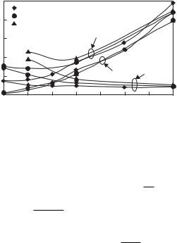
Figure 7.33 Resistance components of a folded MLA ([13], copyright C 2004 IEICE).
where Rl is the loss resistance of a conductor with skin depth δ and conductivity σ , and is given by
√
Rl = δσ . |
(7.33) |
√
Here δ equals f π μ/σ . Then, RL is expressed by
RL = La |
f π μ/2(d + t)√ |
|
. |
(7.34) |
σ |
Here, La is the line length (when extended). The resistance components of a folded meander line antenna with respect to the antenna length L/λ are shown in Figure 7.33, in which the radiation resistance Rr, the loss resistance RL, and input resistance Rin, are depicted for cases N = 10, 22, and 38, and d = 0.3 mm. RL is calculated simply from
RL = Rin − Rin(σ = ∞). |
(7.35) |
It is shown in the figure that, as the antenna length L becomes shorter, the loss resistance RL increases, suggesting decrease in the radiation efficiency. It is also observed from the figure by comparing with the resistance components of a dipole type shown before in Figure 7.28 that a folded type exhibits greater resistance components than the dipole type. Rres is about four times greater than that of the dipole type, showing the stepping-up effect due to the folded structure. The loss resistance RL is, however, not four times, but only about two times, and yet increases when the antenna length becomes shorter. This is because of RL dependence on the line length La, which increases with increase in N. Rin, on the contrary, decreases rapidly as the antenna length L becomes shorter.
The radiation efficiency η is calculated for both dipole-type and folded-type antennas with respect to the antenna length L/λ, and is depicted in Figure 7.34 for N = 10, 22, and 38. With greater N, the radiation efficiency η rapidly decreases as L becomes smaller, particularly in the dipole type, whereas less variation appears in the folded type.
Trial antennas of length 0.1 λ of both dipole-type and folded-type MLAs are manufactured. The parameters of the folded-type MLA are: N = 10, L = 43 mm (0.1λ),