7.2.1.1.1.4Discussions on small NMHA and meander line antennas pertaining to the antenna performances

Figure 7.65 Shortening factor S2 of the antenna wire length La (extended length) at resonance in relation to the helix radius a/λ and the pitch p/λ for the group B ([21], copyright C 2008 IEICE).

Figure 7.66 Radiation resistance in relation to the helix radius a/λ and the pitch p/λ for the group A ([21], copyright C 2008 IEICE).

Figure 7.67 Radiation resistance in relation to the helix radius a/λ and the pitch p/λ for the group B ([21], copyright C 2008 IEICE).

to 500 MHz, and they are discussed extensively in [26]. In [26], antenna length kh = 0.5 is taken according to the definition of electrically small size, and parameters to achieve self-resonance, which is desired in designing small antennas, are discussed. The antenna dimensional parameters used are antenna length h, which is 6 cm corresponding to 0.08λ at 400 MHz, diameter of NMHA, width of meander line sections, number N of helical windings for a NMHA, number N of segments for a Meander Line Antenna (MLA), the total length of wire (extended length of wire), wire radius, and antenna geometry. The parameters also include antenna effective volume Ve, effective height, and spherical radius r. The effective volume can be written in terms of an effective spherical radius r, which is given by [27]

Here Q is determined by [28]

Q = (ω/2π ) (d RA/dω)2 + (d X A/dω + | X A | /ω)3 (7.47)

where RA and XA are antenna radiation resistance and reactance, respectively. Antenna performances considered are resonance frequency, Q as a parameter to indicate bandwidth, and resonant radiation resistance. In discussion, the effective volume of spherical radius r is used as a parameter that relates with Q and discussed by using normalized r with the effective height h; that is, r/h.

To lower the resonance frequency in NMHA, one way is to increase the number of windings N of the helix as shown in Figure 7.68, which depicts three models: NMHA

Table 7.2 The physical properties of the three NMHA models ([26], Copyright C 2004 IEEE)

z z z

Figure 7.68 Three models of NMHA with different number of winding N ([26], copyright C 2004 IEEE).

1 to NMHA 3. Here the wire diameter is 0.5 mm. The total wire length also increases and the resonance frequency is lowered from 408.2 MHz to 278 MHz as Table 7.1 and Table 7.2 describe. Radiation resistance and Q also decrease.

In the case of MLA, one way of lowering the resonance frequency is the same as in NMHA; that is, increase the number of meander line segments, thus increasing the total wire length as shown in Figure 7.69, and Table 7.3, which describes increase in the total wire length in models M1 to M2.

Another way is to increase the width of meander line segments as shown also in Figure 7.69, which depicts models M3 and M4 with wider width. In this case, the total length of M3 is decreased from that of M2, but the effective volume is increased so that

132Design and practice of small antennas I

Table 7.3 The physical properties of the six MLA models ([26], copyright C 2004 IEEE)

z z z z

Figure 7.69 MALs with different number of segment and width ([26], copyright C 2004 IEEE).

Figure 7.70 Comparison of NMHAs and MLAs in terms of the width ([26], copyright C 2004 IEEE).

the effective capacitance against the ground is increased. In addition, increase in the effective diameter decreases capacitances between the meander line segments, which results in increase in the effective self-inductance of the wire. These effects contribute to lowering the resonance frequency. This is also the case with models M3 and M4, where the total wire length is kept the same, while the width is increased as is described in Table 7.3. As a consequence, the resonance is lowered.

An MLA is compared with an NMHA at the same resonance frequency of 408 MHz, taking models of NMHA 1, NMHA 4, M6, and M5 (Figure 7.70) as examples. Table 7.4 provides comparisons of the physical and radiation properties of these models. With increase in the width, the total wire length increases in M6 from that of NMHA 1, whereas keeping the same width, that of NMHA 4 increases as compared with that of

Table 7.4 The radiation properties of the two NMHA models and two MLA models ([26], copyright C 2004 IEEE)

H5 H6

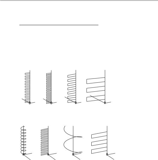
Figure 7.71 NMHAs with different number of turns ([26], copyright C 2004 IEEE).

M5. Radiation resistance decreases in M6 as compared with that of NMHA 1, while a small increase is observed in M5 from NMHA 4. Q and r/h are equal or almost equal regardless of models, NMHA 1, NMHA 4, M6, and M5. The numerical values of these are also given in Table 7.4.

When diameter of the NMHA is increased as shown in Figure 7.71, the total wire length and also the number of turns becomes smaller for the same resonance frequency (fixed at 408 MHz). The physical properties and resonance properties for models H1 to H6 are given in Table 7.5 and Table 7.6, respectively.

When antennas have the same effective height and volume, their resonance properties are essentially identical, independently of any differences in their total wire length and their geometry. The above discussions are useful for designing MLAs and NMHAs.